Chapter 5
Regression Methods
Abstract
This chapter covers two of the most popular function-fitting algorithms. The first is the well-known linear regression method used commonly for numeric prediction. We describe briefly the basics of regression and explain with the classic Boston Housing data set how to implement linear regression in RapidMiner. We also include a discussion on feature selection and provide some checkpoints for correctly implementing linear regression. The second is the more recent logistic regression method used for classification. We explain the basic concepts behind calculation of the logit and how this is used to transform a discrete label variable into a continuous function so that function-fitting methods may be applied. We close with two methods of implementing logistic regression using RapidMiner and show how to use the MetaCost operator to improve the performance of a classification method (such as logistic regression).
Keywords
Linear regression; feature selection; regression model validity; logistic regression; logit; function fittingIn this chapter, we will explore one of the most commonly used predictive analytics techniques—fitting data with functions or function fitting. The basic idea behind function fitting is to predict the value (or class) of a dependent variable y, by combining the predictor variables X into a function, y = f(X). Function fitting involves many different techniques and the most common ones are linear regression for numeric prediction and logistic regression for classification. These two form the majority of material in this chapter. According to an annual survey1 on data mining, regression models continue to be one of the three most common analytics tools used today by practitioners (the others being decision trees and clustering).
Regression is a relatively “old” technique dating back to the Victorian era (1830s to early 1900s). Much of the pioneering work was done by Sir Francis Galton, a distant relative of Charles Darwin, who came up with the concept of “regressing toward the mean” while systematically comparing children’s heights against their parents’ heights. He observed there was a strong tendency for tall parents to have children slightly shorter than themselves, and for short parents to have children slightly taller than themselves. Even if the parents’ heights were at the tail ends of a bell curve or normal distribution, their children’s heights tended toward the mean of the distribution. Thus in the end, all the samples “regressed” toward a population mean. Therefore, this trend was called “regression” by Galton (Galton, 1888) and thus laid the foundations for linear regression
In the first section of this chapter we will provide the theoretical framework for the simplest of function-fitting methods: the linear regression model. Considering its widespread use and familiarity, we will not spend too much time discussing the theory behind it. Instead we will focus more on a case study and demonstrate how to build regression models. Due to the nature of the function fitting approach, a limitation that modelers have to deal with is the “curse of dimensionality.” As the number of predictors X, increases, not only will our ability to obtain a good model reduce, it also adds computational and interpretational complexity. We will introduce feature selection methods that can reduce the number of predictors or factors required to a minimum and still obtain a good model. We will explore the mechanics of using RapidMiner to do the data preparation, model building, and validation. Finally, in closing we will describe some checkpoints to ensure that linear regression is used correctly.
In the second section of this chapter we will discuss logistic regression. Strictly speaking, it is a classification technique, closer in its application to decision trees or Bayesian methods. But it shares an important characteristic with linear regression in its function-fitting methodology and thus merits inclusion in this chapter, rather than the previous one on classification.
We start by discussing how it is different from linear regression and when it makes sense to use it. We will then discuss logistic regression and its implementation using RapidMiner for a simple business analytics application. We will highlight the differences in the implementation of logistic regression in RapidMiner compared to other common tools. Finally, we will spend some time on explaining how to use a costing operator to selectively weight misclassifications while using logistic regression.
Predicting home prices vs. explaining what factors affect home prices
What features would play a role in deciding the value of a home? For example, the number of rooms, its age, the quality of schools, its location with respect to major sources of employment, and its accessibility to major highways are some of the important considerations most potential home buyers would like to factor in. But which of these are the most significant influencers of the price? Is there a way to determine these? Once we know them, can we incorporate these factors in a model that can be used for predictions? The case study we discuss a little later in this chapter addresses this problem using multiple linear regression to predict the median home prices in an urban region given the characteristics of a home.
A common goal that all businesses have to address in order to be successful is growth, in revenues and profits. Customers are what will enable this to happen. Understanding and increasing the likelihood that someone will buy again from the company is therefore critical. Another question that would help strategically, for example in customer segmentation, is being able to predict how much money a customer is likely to spend, given data about their previous purchase habits. Two very important distinctions need to be made here: understanding why someone purchased from the company will fall into the realm of explanatory modeling whereas predicting how much someone is likely to spend will fall into the realm of predictive modeling. Both these types of models fall under a broader category of “Surrogate” or empirical models that rely on historical data to develop rules of behavior as opposed to “System” models which use fundamental principles (such as laws of physics or chemistry) to develop rules. See Figure 1.2 for a taxonomy of Data Mining. In this chapter, we focus on the predictive capability of models as opposed to the explanatory capabilities. Much of applied linear regression history of statistics has been used for explanatory needs. We will show with an example, for the case of logistic regression, how both needs can be met with good analytical interpretation of models.

5.1. Linear Regression
5.1.1. How it Works
Linear regression is not only one of the oldest predictive methodologies, but it also the most easily explained method for demonstrating function fitting. The basic idea is to come up with a function that explains and predicts the value of the target variable when given the values of the predictor variables. A simple example is shown in Figure 5.1: we would like to know the effect of the number of rooms in a house (predictor) on its median sale price (target). Each data point in the chart corresponds to a house (Harrison, 1978). We can see that on average, increasing the number of rooms tends to also increase median price. This general statement can be captured by drawing a straight line through the data. The problem in linear regression is therefore to find a line (or a curve) that best explains this tendency. If we have two predictors, then the problem is to find a surface (in a three-dimensional space). With more than two predictors, visualization becomes impossible and we have to revert to a general statement where we express the dependent (target) variable as a linear combination of independent (predictor) variable:

![]() (5.1)
(5.1)
Let’s consider a problem with one predictor. Clearly we can fit an infinite number of straight lines through a given set of points such as the ones shown in Figure 5.1. How do we know which one is the best? We need a metric that helps to quantify the different straight line fits through the data. Once we find this metric, then selecting the best line becomes a matter of finding the optimum value for this quantity.
A commonly used metric is the concept of an error function. Let’s suppose we fit a straight line through the data. In a single predictor case, the predicted value, ŷ, for a value of x that exists in the data set is then given by
![]() (5.2)
(5.2)
Then, error is simply difference between the actual target value and predicted target value:
![]() (5.3)
(5.3)
This equation defines the error at a single location (x, y) in the data set. We could easily compute the error for all existing points to come up with an aggregate error. Some errors will be positive and others will be negative. We could square the difference to eliminate the sign bias and calculate an average error for a given fit as follows:
![]() (5.4)
(5.4)
where n represents the number of points in the data set. For a given data set, we can then find the best combination of (b0, b1) that minimizes the error, e. This is a classical minimization problem, which is handled by methods of calculus. Stigler provides some interesting historical details on the origins of the method of least squares, as it is known (Stigler, 1999). It can be shown that b1 is given by
![]() (5.5a)
(5.5a)
b0 = ymean - b1∗xmean(5.5b)
where Cor(x,y) is the correlation between x and y (or y and x) and sd(y), sd(x) are the standard deviations of y and x.Finally, xmean and ymean are the respective mean values.
Practical linear regression algorithms use an optimization technique known as gradient descent (Marquardt, 1963; Fletcher, 1963) to identify the combination of b0 and b1 that will minimize the error function given in Equation 5.4. The advantage of using such methods is that even with several predictors, the optimization works fairly robustly. When we apply such a process to the simple example shown above, we get an equation of the form
![]() (5.6)
(5.6)
where b1 is 9.1 and b0 is –34.7. From this equation, we can calculate that for a house with six rooms, the value of the median price is about 20 (the prices are expressed in thousands of dollars). From Figure 5.1 we see that for a house with six rooms, the actual price can range between 10.5 and 25. We could have fit an infinite number of lines in this band, which would have all predicted a median price within this range—but the algorithm chooses the line that minimizes the average error over the full range of the independent variable and is therefore the best fit for the given dataset.
For some of the points (houses) shown in Figure 5.1 (at the top of the chart, where median price = 50) the median price appears to be independent of the number of rooms. This could be because there may be other factors that also influence the price. Thus we will need to model more than one predictor and will need to use multiple linear regression (MLR), which is an extension of simple linear regression. The algorithm to find the coefficients of the regression equation 5.1 can be easily extended to more than one dimension.
MLR can be applied in any situation where a numeric prediction, for example “how much will something sell for,” is required. This is in contrast to making categorical predictions such as “will someone buy/not buy” and “will fail/will not fail,” where we use classification tools such as decision trees (Chapter 4) or logistic regression models (Section 5.4). In order to ensure regression models are not arbitrarily deployed, we must perform several checks on the model to ensure that the regression is accurate. This is discussed in more detail in Section 5.3.
5.1.2. Case Study in RapidMiner: Objectives and Data
Let us extend the housing example introduced earlier in this chapter to include additional variables. This comes from a study of urban environments conducted in the late 1970s (Harrison, 1978). The full data set and information are available in many public databases.2 The objectives of this exercise are:
1. Identify which of the several attributes are required to accurately predict the median price of a house.
2. Build a multiple linear regression model to predict the median price using the most important attributes.
The original data consists of thirteen predictors and one response variable, which is the variable we are trying to predict. The predictors include physical characteristics of the house (such as number of rooms, age, tax, and location) and neighborhood features (school, industries, zoning) among others–refer to the original data source for full details. The response variable is of course the median value (MEDV) of the house in thousands of dollars. Table 5.1 shows a snapshot of the data set, which has altogether 506 examples. Table 5.2 describes the features or attributes of the data set.
Table 5.1
Sample view of the classic Boston Housing data set
| CRIM | ZN | INDUS | CHAS | NOX | RM | AGE | DIS | RAD | TAX | PTRATIO | B | LSTAT | MEDV |
| 0.00632 | 18 | 2.31 | 0 | 0.538 | 6.575 | 65.2 | 4.09 | 1 | 296 | 15.3 | 396.9 | 4.98 | 24 |
| 0.02731 | 0 | 7.07 | 0 | 0.469 | 6.421 | 78.9 | 4.9671 | 2 | 242 | 17.8 | 396.9 | 9.14 | 21.6 |
| 0.02729 | 0 | 7.07 | 0 | 0.469 | 7.185 | 61.1 | 4.9671 | 2 | 242 | 17.8 | 392.83 | 4.03 | 34.7 |
| 0.03237 | 0 | 2.18 | 0 | 0.458 | 6.998 | 45.8 | 6.0622 | 3 | 222 | 18.7 | 394.63 | 2.94 | 33.4 |
| 0.06905 | 0 | 2.18 | 0 | 0.458 | 7.147 | 54.2 | 6.0622 | 3 | 222 | 18.7 | 396.9 | 5.33 | 36.2 |
| 0.02985 | 0 | 2.18 | 0 | 0.458 | 6.43 | 58.7 | 6.0622 | 3 | 222 | 18.7 | 394.12 | 5.21 | 28.7 |
| 0.08829 | 12.5 | 7.87 | 0 | 0.524 | 6.012 | 66.6 | 5.5605 | 5 | 311 | 15.2 | 395.6 | 12.43 | 22.9 |
| 0.14455 | 12.5 | 7.87 | 0 | 0.524 | 6.172 | 96.1 | 5.9505 | 5 | 311 | 15.2 | 396.9 | 19.15 | 27.1 |

Table 5.2
Attributes of Boston Housing Data Set
1. CRIM per capita crime rate by town
2. ZN proportion of residential land zoned for lots over 25,000 sq.ft.
3. INDUS proportion of nonretail business acres per town
4. CHAS Charles River dummy variable (= 1 if tract bounds river; 0 otherwise)
5. NOX nitric oxides concentration (parts per 10 million)
6. RM average number of rooms per dwelling
7. AGE proportion of owner-occupied units built prior to 1940
8. DIS weighted distances to five Boston employment centers
9. RAD index of accessibility to radial highways
10. TAX full-value property-tax rate per $10,000
11. PTRATIO pupil-teacher ratio by town
12. B 1000(Bk – 0.63)^2 where Bk is the proportion of blacks by town
13. LSTAT % lower status of the population
14. MEDV Median value of owner-occupied homes in $1000’s
5.1.3. How to Implement
In this section, we will show how to set up a RapidMiner process to build a multiple linear regression model for the Boston Housing dataset. We will describe the following:
1. Building a linear regression model
2. Measuring the performance of the model
3. Understanding the commonly used options for the Linear Regression operator
4. Applying the model to predict MEDV prices for unseen data
Step 1: Data Preparation
As a first step, let us separate the data into a training set and an “unseen” test set. The idea is to build the model with the training data and test its performance on the unseen data. With the help of the Retrieve operator, import the raw data into the RapidMiner process (refer to Chapter 13 for details on loading data). Apply the Shuffle operator to randomize the order of the data so that when we separate the two partitions, they are statistically similar. Next, using the Filter Examples Range operator, divide the data into two sets as shown in Figure 5.2. The raw data has 506 examples, which will be linearly split into a training set (from row 1 to 450) and a test set (row 451 to 506) using the two operators.
Insert the Set Role operator, change the role of MEDV to “label” and connect the output to a Split Validation operator’s input “tra” or training port as shown in Figure 5.3. The training data is now going to be further split into a training set and a validation set (keep the default Split Validation options as is, i.e., relative, 0.7, and shuffled). This will be needed in order to measure the performance of the linear regression model. It is also a good idea to set the local random seed (to default the value of 1992), which ensures that RapidMiner selects the same samples if we run this process at a later time.


After this step, double-click the Validation operator to enter the nested process. Inside this process insert the Linear Regression operator on the left window and Apply Model and Performance (Regression) in the right window as shown in Figure 5.4. Click on the Performance operator and check “squared error,” “correlation,” and “squared correlation” inside the Parameters options selector on the right.
Step 2: Model Building
Select the Linear Regression operator and change the “feature selection” option to “none.” Keep the default “eliminate collinear features” checked, which will remove factors that are linearly correlated from the modeling process. When two or more attributes are correlated to one another, the resulting model will tend to have coefficients that cannot be intuitively interpreted and furthermore the statistical significance of the coefficients also tends to be quite low. Also keep the “use bias” checked to build a model with an intercept (the b0 in Equation 5.2). Keep the other default options intact (Figure 5.5).
When we run this process we will generate the results shown in Figure 5.6 (assuming that the “mod” and “ave” output ports from the Validation operator are connected to the main output port): a Linear Regression model and an average Performance Vector output of the model on the validation set.


Step 3: Execution and Interpretation
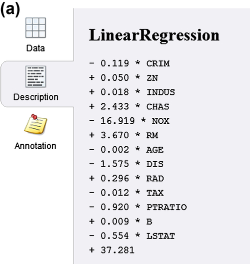
There are two views that you can examine in the Linear Regression output tab: the Description view, which actually shows the function that is fitted (Figure 5.6a) and the more useful Data view, which not only shows the coefficients of the linear regression function, but also gives information about the significance of these coefficients (Figure 5.6b). The best way to read this table is to sort it by double-clicking on the column named “Code,” which will sort the different factors according to their decreasing level of significance. RapidMiner assigns four stars (∗∗∗∗) to any factor that is highly significant.
In this model we did not use any feature selection method (see Figure 5.5) and as a result all 13 factors are in the model, including AGE and INDUS, which have very low significance; see the Text view in Figure 5.7a. However, if we were to run the same model by selecting any of the options that are available in the drop-down menu of the feature selection parameter (see Figure 5.5), RapidMiner would have removed the least significant factors from the model. In the next iteration, we use the greedy feature selection and this has removed the least significant factors, INDUS and AGE, from the function as seen in Figure 5.7b. Notice that the intercept and coefficients are slightly different for the new model.


Feature selection in RapidMiner can be done automatically within the Linear Regression operator as described above or by using external “wrapper” functions such as forward selection and backward elimination. These will be discussed separately in Chapter 12.
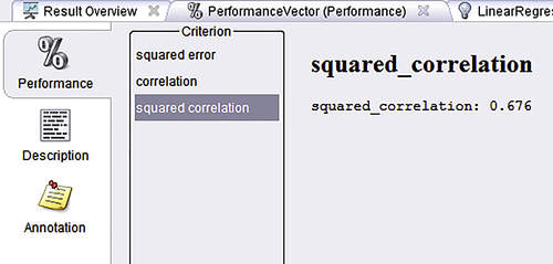

The second output to pay attention to is the Performance: a handy check to test the goodness of fit in a regression model is the squared correlation. Conventionally this is the same as the adjusted R2 for a model, which can take values between 0.0 and 1.0, with values closer to 1 indicating a better model. For either of the models shown above, we get a value around 0.67 (Figure 5.8). We also requested the squared error output: the raw value in itself may not tell us much, but this is useful in comparing two different models. In this case it was around 25.
One additional insight we can extract from the modeling process is ranking of the factors. The easiest way to check this is to rank by p-value. As seen in Figure 5.9, RM, LSTAT, and DIS seem to be the most significant factors. This is also reflected in their absolute t-stat values. The t-stat and p-values are the result of the hypothesis tests conducted on the regression coefficients. For the purposes of predictive analysis, the key takeaway is that a higher t-stat signals that the null hypothesis—which assumes that the coefficient is zero—can be safely rejected. The corresponding p-value indicates the probability of wrongly rejecting the null hypothesis. We already saw how the number of rooms (RM) was a good predictor of the home prices, but it was unable to explain all of the variations in median price. The R2 and squared error for that one-variable model were 0.405 and 45, respectively. You can verify this by rerunning the model built so far using only one independent variable, the number of rooms, RM. This is done by using the Select Attributes operator, which has to be inserted in the process before the Set Role operator. When this model is run, we will obtain the equation shown earlier, Equation 5.6, in the model Description. By comparing the corresponding values from the MLR model (0.676 and 25) to the simple linear regression model, we see that both of these quantities have improved, thus affirming our decision to use multiple factors.
We now have a more comprehensive model that can account for much of the variability in the response variable, MEDV. Finally, a word about the sign of the coefficients: LSTAT refers to the percentage of low-income households in the neighborhood. A lower LSTAT is correlated with higher median home price, and this is the reason for the negative coefficient on LSTAT.
Step 4: Application to Unseen Test Data
We are now ready to deploy this model against the “unseen” data that was created at the beginning of this section using the second Filter Examples operator (Figure 5.2). We need to add a new Set Role operator, select MEDV under parameters and set it to target role “prediction” from the pull-down menu. Add another Apply Model operator and connect the output of Set Role to its “unl” or unlabeled port; additionally connect the output “mod”from the Validation process to the input “mod” or model port of the new Apply Model. What we have done is to change the attribute MEDV from the unseen set of 56 examples to a “prediction.” When we apply the model to this example set, we will be able to compare the prediction (MEDV) values to the original MEDV values (which exist in our set) to test how well our model would behave on new data. The difference between prediction (MEDV) and MEDV is termed “residual.” Figure 5.10 shows one way to quickly check the residuals for our model application. We would need a Rename operator to change the name of “prediction (MEDV)” to “predictedMEDV” to avoid confusing RapidMiner when we use the next operator, Generate Attributes, to calculate residuals (the reader must try without using the Rename operator to understand this issue as it can pop up in other instances where Generate Attributes is used). Figure 5.11 shows the statistics for this new attribute “residuals” which indicate that the mean is close to 0 (–0.275) but the standard deviation (and hence variance) at 4.350 is not quite small. The histogram also seems to indicate that the residuals are not quite normally distributed, which would be another motivation to continue to improve the model.


5.1.4. Checkpoints to Ensure Regression Model Validity
We will close this section on linear regression by briefly discussing several checkpoints to ensure that models are valid. This is a very critical step in the analytics process because all modeling follows the GIGO dictum of “garbage in, garbage out.” It is incumbent upon the analyst to ensure these checks are completed.
Checkpoint 1: One of the first checkpoints to consider before accepting any regression model is to quantify the R2, which is also known as the “coefficient of determination.” R2 effectively explains how much variability in the dependent variable is explained by the independent variables (Black, 2008). In most cases of linear regression the R2 value lies between 0 and 1. The ideal range for r2 varies across applications; for example, in social and behavioral science models typically low values are acceptable. Generally, very low values ( ∼ < 0.2) indicate that the variables in your model do not explain the outcome satisfactorily. A word of caution about overemphasizing the value of R2: When the intercept is set to zero (in RapidMiner, when you uncheck “use bias,” Figure 5.5), R2 values tend to be inflated because of the manner in which they are calculated. In such situations where you are required to have a zero intercept, it makes sense to use other checks such as the mean and variance of the residuals.
Checkpoint 2: This brings us to the next check, which is to ensure that all error terms in the model are normally distributed. To do this check in RapidMiner, we could have generated a new attribute called “error,” which is the difference between the predicted MEDV and the actual MEDV in the test data set. This can be done using the Generate Attributes operator. This is what we did in step 5 in the last section. Passing checks 1 and 2 will ensure that the independent and dependent variable are related. However this does not imply that the independent variable is the cause and the dependent is the effect. Remember that correlation is not causation!
Checkpoint 3: Highly nonlinear relationships will result in simple regression models failing the above checks. However, this does not mean that the two variables are not related. In such cases it may become necessary to resort to somewhat more advanced analytical methods to test the relationship. This is best described and motivated by Anscombe’s quartet, presented in Chapter 3 Data Exploration.
5.2. Logistic Regression
From a historical perspective, there are two main classes of predictive analytics techniques: those that evolved (Cramer, 2002) from statistics (such as regression) and those that emerged from a blend of statistics, computer science, and mathematics (such as classification trees). Logistic regression arose in the mid-twentieth century as a result of the simultaneous development of the concept of the logit in the field of biometrics and the advent of the digital computer, which made computations of such terms easy. So to understand logistic regression, we need to explore the logit concept first. The chart in Figure 5.12, adapted from data shown in Cramer (2002) shows the evolving trend from initial acceptance of the logit concept in the mid-1950s to the surge in references to this concept toward the latter half of the twentieh century. The chart is an indicator of how important logistic regression has become over the last few decades in a variety of scientific and business applications.
5.2.1. A Simple Explanation of Logistic Regression
To introduce the logit, we will consider a simple example. Recall that linear regression is the process of finding a function to fit the x’s that vary linearly with y with the objective of being able to use the function as a model for prediction. The key assumptions here are that both the predictor and target variables are continuous, as seen in the chart in Figure 5.13. Intuitively, one can state that when x increases, y increases along the slope of the line.


What happens if the target variable is not continuous? Suppose our target variable is the response to advertisement campaigns—if more than a threshold number of customers buy for example, then we consider the response to be 1; if not the response is 0. In this case, the target (y) variable is discrete (as in Figure 5.14); the straight line is no longer a fit as seen in the chart. Although we can still estimate—approximately—that when x (advertising spend) increases, y (response or no response to a mailing campaign) also increases, there is no gradual transition; the y value abruptly jumps from one binary outcome to the other. Thus the straight line is a poor fit for this data.
On the other hand, take a look at the S-shaped curve in Figure 5.15. This is certainly a better fit for the data shown. If we then know the equation to this “sigmoid” curve, we can use it as effectively as we used the straight line in the case of linear regression.
Logistic regression is thus the process of obtaining an appropriate nonlinear curve to fit the data when the target variable is discrete. How is the sigmoid curve obtained? How does it relate to the predictors?


5.2.2. How It Works
Let us reexamine the dependent variable, y. If it is binomial, that is, it can take on only two values (yes/no, pass/fail, respond/does not respond, and so on), then we can encode y to assume only two values: 1 or 0. Our challenge is to find an equation that functionally connects the predictors, x, to the outcome y where y can only take on two values: 0 or 1. However ,the predictors themselves may have no restrictions: they could be continuous or categorical. Therefore, the functional range of these unrestricted predictors is likely to be also unrestricted (between –∞ to +∞). To overcome this problem, we must map the continuous function to a discrete function. This is what the logit helps us to achieve.
How Does Logistic Regression Find the Sigmoid Curve?
As we observed in Equation 5.1, a straight line can be depicted by only two parameters: the slope (b1) and the intercept (b0). The way in which x’s and y are related to each other can be easily specified by b0 and b1. However an S-shaped curve is a much more complex shape and representing it parametrically is not as straightforward. So how does one find the mathematical parameters to relate the x’s to the y?
It turns out that if we transform the target variable y to the logarithm of the odds of y, then the transformed target variable is linearly related to the predictors, x. In most cases where we need to use logistic regression, the y is usually a yes/no type of response. This is usually interpreted as the probability of an event happening (y = 1) or not happening (y = 0). Let us deconstruct this as follows:
▪ If y is an event (response, pass/fail, etc.),
▪ and p is the probability of the event happening (y = 1),
▪ then (1 – p) is the probability of the event not happening (y = 0),
▪ and p/(1 – p) are the odds of the event happening.
The logarithm of the odds, log (p/1 – p) is linear in the predictors, X, and log (p/1 – p) or the log of the odds is called the logit function.
We can express the logit as a linear function of the predictors X, similar to the linear regression model shown in Equation 5.1 as
![]() (5.7)
(5.7)
For a more general case, involving multiple independent variables, x, we have
![]() (5.8)
(5.8)
The logit can take any value from –∞ to +∞. For each row of predictors in a data set, we can now compute the logit. From the logit, it is easy to then compute the probability of the response y (occurring or not occurring) as seen below:
![]() (5.9)
(5.9)
The logistic regression model from Equation 5.8 ultimately delivers the probability of y occurring (i.e., y = 1), given specific value(s) of X via Equation 5.9. In that context, a good definition of logistic regression is that it is a mathematical modeling approach in which a best-fitting, yet least-restrictive model is selected to describe the relationship between several independent explanatory variables and a dependent binomial response variable. It is least restrictive because the right side of Equation 5.8 can assume any value from –∞ to +∞. Cramer (2002) provides more background on the history of the logit function.
From the data given we know the x’s and using Equations 5.8 and 5.9 we can compute the p for any given x. But to do that, we first need to determine the coefficients, b, in Equation 5.8. How is this done? Let us assume that we start out with a trial of values for b. Given a training data sample, we can compute the following quantity:

where y is our original outcome variable (which can take on 0 or 1) and p is the probability estimated by the logit equation (Equation 5.9). For a specific training sample, if the actual outcome was y = 0 and our model estimate of p was high (say 0.9), i.e., the model was “wrong,” then this quantity reduces to 0.1. If the model estimate of probability was low (say 0.1), i.e., the model was “good,” then this quantity increases to 0.9. Therefore, this quantity, which is a simplified form of a likelihood function, is maximized for good estimates and minimized for poor estimates. If we compute a summation of the simplified likelihood function across all the training data samples, then a high value indicates a good model (or good fit) and vice versa.
In reality, nonlinear optimization techniques are used (methods such as a generalized reduced gradient search) to search for the coefficients, b, with the objective of maximizing the likelihood of correct estimation (or py ∗ (1 – p)(1 – y), summed over all training samples). More sophisticated formulations of likelihood estimators are used in practice (Eliason, 1993). Assuming we have used a software package like RapidMiner to perform this optimization to generate a model, let us examine how to interpret and apply the model. In the next section, we will walk through a step-by-step process to build the model using RapidMiner.
A Simple but Tragic Example
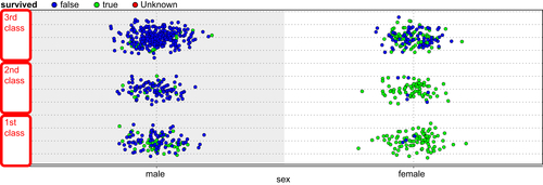
In the 1912 shipwreck of the HMS Titanic, hundreds of people perished as the ship struck an iceberg in the North Atlantic (Hinde, 1998). When we dispassionately analyze the data, we see a couple of basic patterns emerge. 75% of the women and 63% of first class passengers survived. If a passenger was a woman and if she traveled first class, her probability of survival was 97%! The scatterplot in Figure 5.16 below depicts this in an easy to understand way (see the bottom right cluster).
A data mining competition used the information from this event and challenged analysts to develop an algorithm that could classify the passenger list into survivors and nonsurvivors (see http://www.kaggle.com/c/titanic-gettingStarted). We use the training data set provided there as an example3 to demonstrate how logistic regression could be employed to make this prediction and also to interpret the coefficients from the model.
Table 5.3 shows part of a reduced data set consisting only of three variables: travel class of the passenger (pclass = 1st, 2nd, or 3rd), sex of the passenger (0 for male and 1 for female), and the label variable “survived” (true or false). When we fit a logistic regression model to this data consisting of 891 samples, we get the following equation for predicting the class “survived = false” (the details of a generic setup process will be described in the next section):
![]() (5.10)
(5.10)
Comparing this to Equation 5.8, we see that b0 = –0.6503, b1 = –2.6417, and b2 = 0.9595. How do we interpret these coefficients? In order to do this, we need to recall Equation 5.9,
![]()
which indicates that as logit increases to a large positive quantity, the probability that the passenger did not survive (survived = false) approaches 1. More specifically, when logit approaches –∞, p approaches 0 and when logit approaches +∞, p approaches 1. The negative coefficient on variable “sex” indicates that this probability reduces for females (sex = 1) and the positive coefficient on variable p indicates that the probability of not surviving (survived = false) increases the higher the number of the travel class. This verifies the intuitive understanding that was provided by the scatterplot shown in Figure 5.16.
We can also examine the “odds” form of the logistic regression model, which is given below:
![]() (5.11)
(5.11)
Recall that logit is simply given by log(odds) and we are essentially dealing with the same equation as Equation 5.10. A key fact to observe is that a positive coefficient in the logit model translates into a coefficient higher than 1 in the odds model (the number 2.6103 in the above equation is e0.9595 and 0.0712 is e−2.6417) and a negative coefficient in the logit model translates into coefficients smaller than 1 in the odds model. Again it is clear that odds of not surviving increases with travel class and reduces with gender = female.
An odds ratio analysis will reveal the value of computing the results in this format. Consider a female passenger (sex = 1). We can calculate the survivability for this passenger if she was in 1st class (pclass = 1) versus if she was in 2nd class as an odds ratio:

Based on the Titanic data set, the odds that a female passenger would not survive if she was in 2nd class increases by a factor of 2.6 compared to her odds if she was in 1st class. Similarly the odds that a female passenger would not survive increases by nearly seven times if she was in 3rd class! In the next section, we discuss the mechanics of logistic regression and also the process of implementing a simple analysis using RapidMiner.
3 All data sets are made available through the companion site for this book.
5.2.3. How to Implement
The data we used comes from an example4 for a credit scoring exercise. The objective is to predict DEFAULT (Y or N) based on two predictors: loan age (business age) and number of days of delinquency. There are 100 samples Table 5.4.
Step 1: Data Preparation
Load the spreadsheet into RapidMiner. Remember to set the DEFAULT column as “Label.” Split the data into training and test samples using the Split Validation operator.
Step 2: Modeling Operator and Parameters
Add the Logistic Regression operator in the “training” subprocess of the Split Validation operator. Add the Apply Model operator in the “testing” subprocess of the Split Validation operator. Just use default parameter values. Add the Performance (Binominal) evaluation operator in the “testing” subprocess of Split Validation operator. Check the Accuracy, AUC, Precision, and Recall boxes in the parameter settings. Connect all ports as shown in Figure 5.17.
Step 3: Execution and Interpretation
Run the model and view results. In particular check for the kernel model, which shows the coefficients for the two predictors and the intercept. The bias (offset) is −1.820 and the coefficients are given by: w[BUSAGE]=0.592 and w[DAYSDELQ]=2.045. Also check the confusion matrix for Accuracy, Precision, and Recall and finally view the ROC curves and check the area under the curve or AUC. Chapter 8 Model Evaluation provides further details on these important performance measures.
The accuracy of the model based on the 30% testing sample is 83%. The ROC curves have an AUC of 0.863. The next step would be to review the kernel model and prepare for deploying this model. Are these numbers acceptable? In particular, pay attention to the class recall (bottom row of the confusion matrix in Figure 5.18). The model is quite accurate in predicting if someone is NOT a defaulter (91.3%), however its performance when it comes to identifying if someone IS a defaulter is questionable. For most predictive applications, the cost of wrong class predictions is not uniform. That is, a false positive (in the above case identifying someone as a defaulter, when they are not) may be less expensive than a false negative (in this above case identifying someone as a nondefaulter, when they actually are). There are ways to weight the cost of misclassification, and RapidMiner allows this thorugh use of the MetaCost operator.


Step 4: Using MetaCost
Nest the Logistic Regression operator inside a MetaCost operator to improve class recall. The MetaCost operator is now placed inside Split Validation operator. Configure the MetaCost operator as shown in Figure 5.19. Notice that false negatives have twice the cost of false positives. The actual values of these costs can be further optimized using an optimization loop—optimization is discussed for general cases in Chapter 13.
When this process is run, the new confusion matrix that results is shown in Figure 5.20. The overall accuracy has not changed much. Note that while the class recall for the Default = Yes class has increased from 57% to 71%, but this has come at the price of reducing the class recall for Default = No from 91% to 87%. Is this acceptable? Again the answer to this comes from examining the actual business costs. More details about interpreting the confusion matrix and evaluating the performance of classification models is provided in Chapter 8 Model Evaluation.

Step 5: Applying the Model to an Unseen Data Set
In RapidMiner, logistic regression is calculated by creating a support vector machine (SVM) with a modified loss function (Figure 5.21). SVMs were introduced in Chapter 4 on classification. That’s the reason why you see support vectors at all (if you want a “standard” logistic regression, you may use the W-Logistic from the Weka extension to RapidMiner). Weka is another open source implementation of data mining algorithms (see http://www.cs.waikato.ac.nz/ml/weka/) and many of these implementations are available within RapidMiner. The Titanic example was analyzed using the W-logistic operator and it is highly recommended for applications where interpreting coefficients is valuable. Furthermore, the Weka operator may be faster for certain applications than the native SVM-based RapidMiner implementation. Refer to Chapter 4 for details on the mechanics and interpretation of an SVM model.
5.2.4. Summary Points for Logistic Regression Modeling
▪ Logistic regression can be considered equivalent to using linear regression for situations where when the target (or dependent) variable is discrete, i.e., not continuous. In principle, the response variable or label is binomial. A binomial response variable has two categories: Yes/No, Accept/Not Accept, Default/Not Default, and so on. Logistic regression is ideally suited for business analytics applications where the target variable is a binary decision (fail/pass, response/no response, etc). In RapidMiner, such variables are called “binominal.”
▪ The above logit gives the odds of the “Yes” event, however if we want probabilities, we need to use the transformed equation below:
![]()
▪ The predictors can be either numerical or categorical for standard logistic regression. However in RapidMiner, the predictors can only be numerical, because it is based on the SVM formulation.
Conclusion
This chapter explored two of the most common function-fitting methods. Function-fitting methods are one of the earliest predictive modeling techniques based on the concept of supervised learning. The multiple linear regression model works with numeric predictors and a numeric label and is thus one of the go-to methods for numeric prediction tasks. The logistic regression model works with numeric or categorical predictors and a categorical (typically, binomial) label. We explained how a simple linear regression model is developed using the methods of calculus and discussed how feature selection impacts the coefficients of a model. We explained how to interpret the significance of the coefficients using the t-stat and p-values and finally laid down several checkpoints one must follow to build good quality models. We then introduced logistic regression by comparing the similar structural nature of the two function-fitting methods. We discussed how a sigmoid curve can better fit predictors to a binomial label and introduced the concept of logit, which enables us to transform a complex function into a more recognizable linear form. We discussed how the coefficients of logistic regression can be interpreted and how to measure and improve the classification performance of the model. We finally ended the section by pointing out the differences between the implementation of standard logistic regression and RapidMiner’s version.
..................Content has been hidden....................
You can't read the all page of ebook, please click here login for view all page.