
Chapter 10
Time Series Forecasting
Abstract
This chapter provides a high-level overview of time series forecasting and related analysis. It starts by pointing out the clear distinction between standard supervised predictive models and time series forecasting models. It provides a basic introduction to the different time series methods, ranging from data-driven moving averages to exponential smoothing, and also discusses model-driven forecasts including polynomial regression and lag-series-based ARIMA methods. Finally it explains how to implement lag-series-based forecasts using the Windowing operation using RapidMiner. It points out that the implementation of time series in RapidMiner is based on a hybrid concept of transforming series data into “cross-sectional” data that is the standard data format for supervised predictive models.
Keywords
Time series forecasting; exponential smoothing; windowing; cross-sectional data; data-driven forecasting; model-based forecastingTime series forecasting is one of the oldest known predictive analytics techniques. Strictly speaking, it has existed and been in widespread use even before the term “predictive analytics” was ever coined!
Up to this point in this book, supervised model building was about collecting data from several different attributes of a system and using these to fit a “function” to predict the desired quantity or target variable. For example, if the “system” was a housing market, the attributes may have been the price of a house, its square footage, number of bedrooms, number of floors, age, and so on. A multiple linear regression model or a neural network model could be built to predict the price (target) variable given the other (predictor) variables. Similarly, purchasing managers may use data from several different commodity prices that influence the final price of a product to “model” the cost of the product. The common thread among these predictive models is that predictors or independent variables that potentially influence a target (price or product cost) are used to predict that target variable. The objective in time series forecasting is slightly different: use historical information about a particular quantity to make forecasts about value of the same quantity in the future. In general, there are two important differences between time series analysis and other supervised predictive models.
First, in time series analysis we are concerned with forecasting a specific variable, given that we know how this variable has changed over time in the past. In all other predictive models discussed so far, the time component of the data was either ignored or was not available. Such data are known as cross-sectional data (Figure 10.1).
Second, we may not be interested in (or might not even have) data for other attributes that could potentially influence the target variable. In other words, independent or predictor variables are not strictly necessary for univariate time series forecasting (but are strongly recommended for multivariate time series).
Such time series forecasting methods are called data-driven forecasting methods, where there is no difference between a predictor and a target. The predictor is also the target variable. Techniques such as time series averaging or smoothing are considered data-driven approaches to time series forecasting.

However, there is also another class of time series forecasting techniques that are known as model-driven forecasting methods. Model-driven techniques are similar to “conventional” predictive models, which have independent and dependent variables, but with a twist: the independent variable is now time. The simplest of such methods is of course a linear regression model of the form
![]() (10.1)
(10.1)
where y(t) is the value of the target variable at time t. Given a training set, we estimate the values of coefficients a and b to forecast future y values. Model-driven techniques can get pretty complicated in the selection of the type of function. Commonly used functions are exponential, polynomial, and power law functions. Most people are familiar with the trend line function in spreadsheet programs, which offer several different function choices. In a nutshell, a model-driven time series forecast differs from a regular function-fitting predictive model in the choice of the independent variable.
A more sophisticated model-driven technique is based on the concept of autocorrelation. Autocorrelation refers to the fact that data from adjacent time periods may be correlated. The most well known among these techniques is ARIMA, which stands for autoregressive integrated moving average; this will be briefly covered in later sections. We will now describe the concepts of time series forecasting using data-driven and model-driven techniques.
Time series analysis can also be broadly classified into descriptive modeling, called time series analysis, and predictive modeling, called time series forecasting. Both of these rely on a technique called decomposition, where the data is split into a trend component, a seasonal component, and a noise component. The trend and seasonality are predictable (and are called systematic components) whereas the noise, by definition, is random (and is called the nonsystematic component). The discussions in this chapter focus only on time series forecasting techniques. For a complete description of time series decomposition, the reader is referred to books dedicated to time series analysis such as Hyndman (2014).
10.1. Data-Driven Approaches
It is helpful to start out with a basic notation system for time series in order to understand the different methodologies. The following measures are important:
▪ Time periods: t = 1, 2, 3, …, n . Time periods can be seconds, days, weeks, months, or years depending on the problem.
▪ Data series corresponding to each time period above: y1, y2, y3, … yn.
▪ Forecasts: Fn+h  forecast for the hth time period following n. Usually h = 1, the next time period following the last data point. However h can be greater than 1. “h” is called the horizon.
▪ Forecast errors: et = yt – Ft for any given time, t.
In order to explain the different methods, we will use a simple time series data function, Y(t). Y is the value of the time series at any time t. The data represents the value of Y over a 36-month period. (Data and accompanying models are available from the companion site www.LearnPredictiveAnalytics.com) As you can see in Figure 10.3, Y(t) can be imagined to be made up of a periodic (or seasonal) component and a random (noise) component. Additionally, Y(t) may have a small (in this case, upward) linear trend as well. Furthermore, the time periods are constant. However, for some data the period may be variable. In such cases, we assume that an interpolation scheme is applied to obtain equally spaced (in time) data points.
10.1.1. Naïve Forecast
Probably the simplest forecasting “model.” Here we simply assume that Fn+1, the forecast for the next period in the series, is given by the last data point of the series, yn:
![]() (10.2)
(10.2)

10.1.2. Simple Average
Moving up a level, we could compute the next data point as an average of all the data points in the series. In other words, this model calculates the forecasted value, Fn+1, as
![]() (10.3)
(10.3)
Suppose we have monthly data from January to December and we want to predict the next January (n + 1) value, we simply average the values from January (n = 1) to December (n = 12).
10.1.3. Moving Average
The obvious problem with a simple average is figuring out how many points to use in the average calculation. As the data grows (as n increases), should we still use all the n time periods to compute the next forecast? To overcome this problem, we can select a window of the last “k” periods to calculate the average, and as the actual data grows over time, we always take the last k samples to average, i.e., n, n – 1, …, n – k + 1. In other words, the window for averaging keeps moving forward and thus returns a moving average. Suppose in our simple example that the window k = 3; then to predict the January data, we take a three-month average using the last three months. When the actual data from January comes in, the February value is forecasted using January (n), December (n – 1) and November (n – 3 + 1 or n – 2). This model will result in problems when there is seasonality in data (for example, in December for retail or in January for healthcare insurance), which can skew the average.
10.1.4. Weighted Moving Average
For some cases, the most recent value could have more influence than some of the earlier values. Most exponential growth occurs due to this simple effect. The forecast for the next period is given by the model
![]() (10.4)
(10.4)
where typically a > b > c. Figure 10.4 compares the forecast results for the simple time series introduced earlier. Note that all of the above methods are able to make only one-step-ahead forecasts due to the nature of their formulation. The coefficients a, b, and c may be arbitrary, but are usually based on some previous knowledge of the time series.
Next we will consider exponential smoothing, which is a slightly different form of weighted moving averages.

10.1.5. Exponential Smoothing
What would happen if we use the previously forecasted value for a given period to predict the value for the next period? Going back to our monthly example, if we wanted to make the February forecast using not only the actual January value but also the previously forecasted January value, the new forecast would have “learned” the data a little better. This is the concept behind basic exponential smoothing (Brown, 1956):
![]() (10.5)
(10.5)
α is generally between 0 and 1. If α is close to 1, then the previously forecasted value of the last period has less weight than the actual value of the last period and vice versa. Note that α = 1 returns the naïve forecast of Equation 10.2. As seen in the charts in Figure 10.5, using a higher α results in putting more weight on actual values and the resulting curve is closer to the actual curve, but using a lower α results in putting more emphasis on previously forecasted value and results in a smoother but less accurate fit. Typical values for α range from 0.2 to 0.4 in practice.
This simple exponential smoothing is the basis for a number of very common data-driven forecasting methods. The above model has only one parameter, α, and can help to smooth the data in a time series so that it is easy to extrapolate and make forecasts. But if you examine Equation 10.5, you see that you cannot make forecasts more than one-step ahead, because to make a forecast for step (n + 1), we need data for the previous step, n. It is not possible to make forecasts several steps ahead, i.e., (n + h), using the three methods described above (where we have simply assumed that Fn+h = Fn+1). Here “h” is called the “horizon.” This obviously has limited utility. For making longer horizon forecasts, that is where h >> 1, we need to also consider trend and seasonality information and the simple exponential smoothing methods quickly become more complicated. An overview of advanced exponential smoothing is described in the next few sections.

A time series is made up of what is known as nonstationary data. “Nonstationary” means that the series typically demonstrates a trend and a seasonal pattern in addition to “normal” fluctuations (Hyndman, 2014). As mentioned earlier, most time series can be decomposed into the following components: trend, seasonality, and random noise (see Figure 10.6). To be able to capture trend and seasonality, we need more sophisticated techniques than the ones described so far. The good news is that there are many well-established data-driven methods that can help accomplish this. Once we capture trend and seasonality, we can forecast the value at any time in the future, not just one step ahead values. We will give a bird’s eye view of the common ones to introduce them.
10.1.6. Holt’s Two-Parameter Exponential Smoothing
Anyone who has used a spreadsheet for creating trend lines on scatterplots intuitively knows what a trend means. A trend is an averaged long-term tendency of a time series. The simplified exponential smoothing model described earlier is not very effective at capturing trends. An extension of this technique called Holt’s two-parameter exponential smoothing is needed to accomplish this.

Recall that exponential smoothing Equation (10.5) simply calculates the average value of the time series at n + 1. If the series also has a trend, then an average slope of the series needs to be estimated as well. This is what Holt’s two-parameter smoothing does by means of another parameter, β. A smoothing equation similar to Equation 10.5 is constructed for the average trend at n + 1. With two parameters, α and β, any time series with a trend can be modeled and therefore forecasted. The forecast can be expressed as a sum of these two components, average value or “level” of the series, Ln, and trend, Tn, recursively as follows:
![]() (10.6)
(10.6)
where, Ln = α ∗ yn + (1 – α) ∗ (Ln–1 + Tn–1) and Tn = β ∗ (Ln – Ln–1) + (1 – β) ∗ Tn–1
10.1.7. Holt-Winters’ Three-Parameter Exponential Smoothing
When a time series contains seasonality in addition to a trend, we will need yet another parameter, γ, to estimate the seasonal component of the time series (Winters, 1960). The estimates for value (or level) are now adjusted by a seasonal index, which is computed with a third equation that includesγ. For mathematical details of all these algorithms, the reader is referred to one of the many texts dedicated to time series forecasting (Shmueli, 2011; Hyndman, 2014; Box, 2008).
10.2. Model-Driven Forecasting Methods
Model-driven approaches to time series forecasting will overcome the one-step-ahead limitation of some of the data-driven methods. As mentioned at the beginning of the chapter, in model-driven methods, time is the predictor or independent variable and the time series value is the dependent variable. Model-based methods are generally preferable when the time series appears to have a “global” pattern. The idea is that the model parameters will be able to capture these patterns and thus enable us to make predictions for any step ahead in the future under the assumption that this pattern is going to repeat. For a time series with local patterns instead of a global pattern, using the model-driven approach requires specifying how and when the patterns change, which is difficult. For such a series, data-driven approaches work best because these methods usually rely on extrapolating the most recent local pattern as we saw earlier.
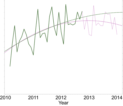
Figure 10.7 shows two time series: Figure 10.7a shows annual monsoon precipitation in Southwest India averaged over a five-year period (Krishnakumar, 2009). Figure 10.7b shows the adjusted month-end closing prices of the SPDR S&P 500 (SPY) Index over another five-year period. Clearly a model-driven forecasting method would work very well for the rainfall series. However the financial time series shows no clear start or end for any patterns. It is preferable to use data-driven methods to attempt to forecast this second series.
10.2.1. Linear Regression
The simplest of the model-driven approaches for analyzing a time series is using linear regression. As mentioned in the introduction to the chapter, we assume the time period is the independent variable and attempt to predict the time series value using this. For the simple 36-month dataset we have used so far, the chart in Figure 10.8a shows a linear regression fit created using a standard spreadsheet. As you can see, the linear regression model is able to capture the long-term tendency of the series, but it does a very poor job of fitting the data. This is reflected in the R2 value shown as well.
10.2.2. Polynomial Regression
We can attempt to improve this using a more “sophisticated” polynomial fit. Polynomial regression is similar to linear regression except that higher-degree functions of the independent variable are used (squares and cubes). As seen in Figure 10.8b, it is difficult to argue that the cubic polynomial does a significantly better job. However in either of these cases, we are not limited to a one-step-ahead forecast of the simple smoothing (data-driven) methods.

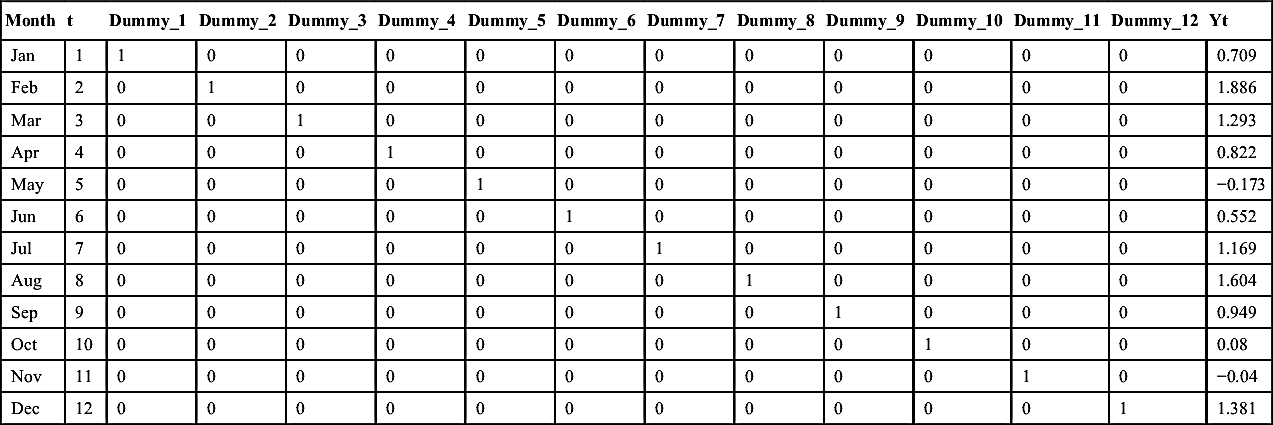
10.2.3. Linear Regression with Seasonality
But one can significantly improve upon the fit with linear regression by simply accounting for seasonality. This is done by introducing dummy variables for each month of the series, which trigger to 1 or 0 as seen in the table in Table 10.1. Just this very trivial addition to the predictors of the linear regression model can yield a surprisingly good fit as seen in Figure 10.9. Although the model equation may appear very complicated, in reality it is just a linear regression model in 13 variables: the time period and 12 dummy variables for each month of a year. The time-independent variable captures the trend and the 12 dummy variables capture seasonality. This regression equation can be used for predicting any future value beyond n + 1, and thus has significantly more utility than the corresponding simpler counterparts in the data-driven side.


Table 10.1
Seasonality Modeled via Linear Regression and the Accompanying Fit
| Month | t | Dummy_1 | Dummy_2 | Dummy_3 | Dummy_4 | Dummy_5 | Dummy_6 | Dummy_7 | Dummy_8 | Dummy_9 | Dummy_10 | Dummy_11 | Dummy_12 | Yt |
| Jan | 1 | 1 | 0 | 0 | 0 | 0 | 0 | 0 | 0 | 0 | 0 | 0 | 0 | 0.709 |
| Feb | 2 | 0 | 1 | 0 | 0 | 0 | 0 | 0 | 0 | 0 | 0 | 0 | 0 | 1.886 |
| Mar | 3 | 0 | 0 | 1 | 0 | 0 | 0 | 0 | 0 | 0 | 0 | 0 | 0 | 1.293 |
| Apr | 4 | 0 | 0 | 0 | 1 | 0 | 0 | 0 | 0 | 0 | 0 | 0 | 0 | 0.822 |
| May | 5 | 0 | 0 | 0 | 0 | 1 | 0 | 0 | 0 | 0 | 0 | 0 | 0 | −0.173 |
| Jun | 6 | 0 | 0 | 0 | 0 | 0 | 1 | 0 | 0 | 0 | 0 | 0 | 0 | 0.552 |
| Jul | 7 | 0 | 0 | 0 | 0 | 0 | 0 | 1 | 0 | 0 | 0 | 0 | 0 | 1.169 |
| Aug | 8 | 0 | 0 | 0 | 0 | 0 | 0 | 0 | 1 | 0 | 0 | 0 | 0 | 1.604 |
| Sep | 9 | 0 | 0 | 0 | 0 | 0 | 0 | 0 | 0 | 1 | 0 | 0 | 0 | 0.949 |
| Oct | 10 | 0 | 0 | 0 | 0 | 0 | 0 | 0 | 0 | 0 | 1 | 0 | 0 | 0.08 |
| Nov | 11 | 0 | 0 | 0 | 0 | 0 | 0 | 0 | 0 | 0 | 0 | 1 | 0 | −0.04 |
| Dec | 12 | 0 | 0 | 0 | 0 | 0 | 0 | 0 | 0 | 0 | 0 | 0 | 1 | 1.381 |
There is of course no reason to use linear regression alone to capture both trend and seasonality. More sophisticated models can easily be built using polynomial equations along with the sine and cosine function to model seasonality. They will achieve the same effect.
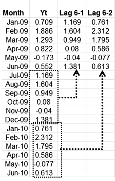
10.2.4. Autoregression Models and ARIMA
The second column of Table 10.2 shows the data for our simple time series. In the third column, we collect the values from month 6 to month 12 of year 1 (2010), and in the fourth column we collect values from month 13 to month 18. This new series of values is termed a “lag ”series and we see that there is some correlation between them. In particular, values belonging to the same row are strongly correlated. For example, every fifth month (May 2010, Nov. 2010, and May 2011), the values drop below zero. This phenomenon is called autocorrelation and it can be used to our advantage. Autoregression methods are basically regression models applied on lag series where each lag series is a new predictor used to fit the dependent variable, which is still the original series value, Yt. In addition to creating a lag series of actual values, we can also create a lag series involving forecast errors and use this as another predictor.
The ARIMA methodology originally developed by Box and Jenkins in the 1970s (Box, 1970) allows us to do this type of modeling. ARIMA is a complex technique and it requires a great deal of experience to produce good forecast results. Although RapidMiner does provide means to perform lagging operations, it does not provide a simple way to implement ARIMA. We refer the reader to the many online and offline resources on ARIMA for further information about its applications (see for example, Alnaa, 2011). In the next few sections we focus on using RapidMiner to perform time series analysis and forecasts.
10.2.5. How to Implement
RapidMiner’s approach to time series is based on two main data transformation processes. The first is windowing to transform the time series data into a generic data set: this step will convert the last row of a window within the time series into a label or target variable. We apply any of the “learners” or algorithms to predict the target variable and thus predict the next time step in the series. A “typical” time series and its transformed structure (after windowing) is conceptually shown in Figure 10.10.
The parameters of the Windowing operator allow changing the size of the windows (shown as vertical boxes in dashed lines, on the left of figure 10.10), the overlap between consecutive windows (also known as step size), and the prediction horizon, which is used for forecasting. The prediction horizon controls which row in the raw data series ends up as the label variable in the transformed series. (For example, in the above example, the prediction horizon is 0, the next section gives more details.) Thus series data are now converted into a generic cross-sectional data set that can be “predicted” with any of the available algorithms in RapidMiner.
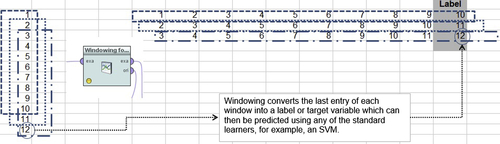
The next main process required for running time series analyses using RapidMiner involves applying any of the available “learners” to “predict” the label variable shown in the gray box (see Figure 10.10). The example set (or raw data) for this learner is the “horizontal” data set shown above with the target or label variable in the box. Also, most of the Performance operators can be used to assess the fitness of the learning scheme to the data.
In this section, we will show how to set up a RapidMiner process to model the simple time series Y(t) described in Section 10.1. The data set could refer to historical monthly profits from a particular product, for example, from January 2009 to June 2010. The data was previously shown in Table 10.1 (column labeled Yt). Our objective in this exercise is to develop profitability forecasts for the next 12 months and also show some of the advantages of using machine learning algorithms for forecasting problems compared to conventional (averaging or smoothing type) forecasting algorithms. The process consists of the following three steps: (1) set up windowing; (2) train the model with several different algorithms; and (3) generate the forecasts.
Step 1: Set Up Windowing
The process window in Figure 10.11 shows the necessary operators for windowing. All time series will have a date column and this must be treated with special care. RapidMiner must be informed that one of the columns in the data set is a date and should be considered as an “id.” This is accomplished by the Set Role operator. If you have multiple commodities in the input data, you may also want to Select Attributes that you want to forecast. In this case, we have only one series and strictly speaking we do not need this operator. However to make the process generic we include it and select the column labeled “inputYt.” The final operator is the Windowing operator. (You may need to install the Series extension, if you have not already. Go to Help -> Manage Extensions to verify.)

Additionally, you may want to use the Filter Examples operator to remove any attributes that have missing values. The main items to consider in Windowing are the following:
▪ Window size: Determines how many “attributes” are created for the cross-sectional data. Each row of the original time series within the window width will become a new attribute. In this example we choose w = 6.
▪ Step size: Determines how to advance the window. Let us use s = 1.
▪ Horizon: Determines how far out to make the forecast. If the window size is 6 and the horizon is 1, then the seventh row of the original time series becomes the first sample for the “label” variable. Let us use h = 1, as well.
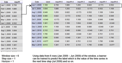
Figure 10.12 shows the original data and the transformed output from the windowing process and describes the transformation details. The main point to keep in mind is that for the window selected and shown in the box the target or response variable value is the value from Jul 1, 2009. When training any algorithm using this data, the attributes labeled inputYt-5 through inputYt-0 form the independent variables. This is shown in the output of step 2 (Figure 10.13).
Step 2: Train the Model
Once the windowing is done, then the real power of predictive analytics algorithms may be brought to bear on a time series analysis. This is where the advantage of using RapidMiner comes into play. Now that the time series is encoded and transformed into a cross-sectional data set, we can use any of the available machine learning algorithms such as regression, neural networks, or support vector machines, for example, to generate predictions. In this case we use linear regression to fit the “dependent” variable called label, given the “independent” variables inputYt-5 through inputYt-0.
Once the model fitting is done, the next step is to start the forecasting process. Note that given this configuration of window size and horizon, we can now only make the forecast for the next step. In the example, the last row of the transformed data set corresponds to Nov. 1, 2011. The independent variables are values from June through November 2011 and the target or label variable is from December 2011. But we can use the regression equation and the values from the Nov. 1, 2011 row to generate the forecast for January 2012. All we need to do is insert the values from July–December into the regression equation to generate the January 2012 forecast. This is just the (n + 1)th forecast and all the sophisticated windowing with equation fitting accomplishes nothing more than what the simple smoothing algorithms described in Section 10.1 could have done! At this point, extending this to provide future values beyond (n + 1) might have become apparent to the reader. Next, we need to generate a new row of data that would run from August–January to predict February using the regression equation. We have all the (actual) data from August to December and the predicted value for January at our disposal. Once we have the predicted February value, there is nothing stopping us from using the actual data from September–December plus predicted January and February values to forecast March.

Actually accomplishing this using RapidMiner is easier said than done. We need to break this up into two separate parts. First, you take the last forecasted row (in this case, December 2011), drop the current value of inputYt-5 (current value is 1.201), rename inputYt-4 to inputYt-5, rename inputYt-3 to inputYt-4, rename inputYt-2 to inputYt-3, rename inputYt-1 to inputYt-2, rename inputYt-0 to inputYt-1, and finally rename predicted label (current value is 1.934) to inputYt-0. With this new row of data, you can then apply the regression model to predict the next date in the series: January 2012. Next, you need to put this entire process inside a Loop operator that will allow you to repeatedly run these steps for as many future periods as you need.

The results of this process are illustrated in Figure 10.14 and the implementation is described in detail in step 3.
Step 3: Generate the Forecasts
The outer level process for the first part is shown in Figure 10.15. We can add another Windowing operator, which will transform input and allow us to collect the last forecasted row and feed it to an inner level Loop process (Figure 10.16). The Loop operator will contain all the mechanisms for accomplishing the renaming and, of course, to perform looping. Set the iterations in the Loop operator to the number of future months to forecast (horizon). In our case, this is defined by a variable called futureMonths whose value can be changed by the user before process execution. It is also possible to capture the Loop counts in a macro if you click the set iteration macro check box. A macro in RapidMiner is nothing but a variable that can be called by other operators in the process. When set iteration macro is checked and a name is provided in the macro name box, a variable will be created with that name whose value will be updated each time, one loop is completed. An initial value for this macro is set by the macro start value option. Loops may be terminated by specifying a timeout, which is enabled by checking the limit time box. A macro variable can be used by any other operator by using the format %{macro name} in place of a numeric value.
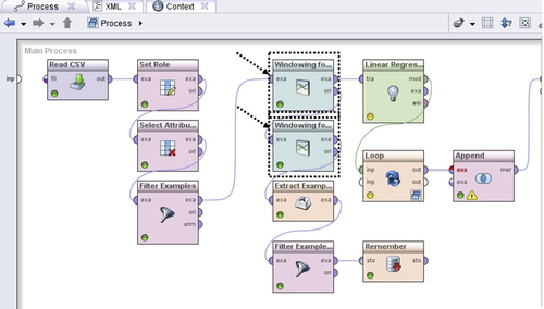
But before we start the looping, we need to store the last forecasted row in a separate data structure. This is accomplished by the macro titled Extract Example Set. The Filter Example operator simply deletes all rows of the transformed data set except the last forecasted row. Finally the Remember operator stores this in memory and allows us to “recall” the stored value once inside the loop.

The loop parameter iterations will determine the number of times the inner process is repeated. During each iteration, the model is applied on the last forecasted row, and bookkeeping operations are performed to prepare application of the model to forecast the next month. This includes incrementing the month (date) by one, changing the role of the predicted label to that of a regular attribute, and finally renaming all the attributes as discussed in the last part of step 2. The newly renamed data is stored and then recalled before the next iteration begins.
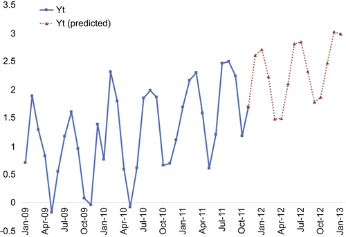
The output of our process is shown in Figure 10.17 as an overlay on top of the actual data. (The tabular form of the results was already shown in Figure 10.14.) As seen, the simple linear regression model seems to adequately capture both the trend and seasonality of the underlying data. The real benefit of using RapidMiner for time series forecasting lies in being able to quickly change the modeling scheme. We can quickly swap out the Linear Regression operator of step 2 to a Support Vector Machine operator and test its performance without having to do any other programming or process modification. Ultimately, the user can select the best performing modeler with very little extra effort.
An important point about any time series forecasting is that one should not place too much emphasis on “point” forecasts. A complex quantity like a stock price or sales demand for a manufactured good is influenced by too many factors and to claim that any forecasting will predict the exact value of a stock two days in advance or the exact value of demand three months in advance is unrealistic. However, what is far more valuable is the fact that recent undulations in the price or demand can be effectively captured and predicted. This is where RapidMiner excels by allowing us to swap modeling techniques and experiment.
Conclusion
In this chapter we have given a high level overview of the field of time series modeling. We started out by illustrating the key differences between predictive models for time series and predictive models for cross-sectional data. We then discussed the two main classes of time series forecasting approaches and showed how RapidMiner uses what may best be termed a “hybrid” approach. We finally demonstrated how to implement a real-world time series modeling and forecasting problem entirely using RapidMiner.
Univariate time series forecasting treats prediction as essentially a single-variable problem, whereas multivariate time series may use many time-concurred series for prediction. If you have a series of points spaced over time, conventional forecasting uses smoothing and averaging to “predict” where the next few points will likely be. However, for complex systems such as the economy or stock market, point forecasts are unreliable because these systems are functions of hundreds if not thousands of variables. What is more valuable or useful is the ability to predict trends, rather than point forecasts. We can predict trends with greater confidence and reliability (i.e., Are the quantities going to trend up or down?), rather than the values or levels of these quantities. For this reason, using different modeling schemes such as artificial neural networks or support vector machines or even polynomial regression can sometimes give highly accurate trend forecasts. With conventional forecasting available in the R extension, we have the option of using a variety of smoothing functions and modeling techniques such as ARIMA.
If you do have a time series that is not highly volatile (and therefore more predictable), conventional time series forecasting can help you understand the underlying structure of the variability better. In such cases, trends or seasonal components have a stronger signature than the random component. R does a very good job of taking any time series and breaking it up into these components. If your time series project involves decomposing data into trends and seasonality, then using the R extension in RapidMiner may be the best way to go.
..................Content has been hidden....................
You can't read the all page of ebook, please click here login for view all page.