
Chapter 13
Getting Started with RapidMiner
Abstract
The final chapter is the kickstarter for the main tools that one would need to become familiar with in building predictive analytics models using RapidMiner. We start out by introducing the basic graphical user interface for the program and cover the basic data exploration, transformation, and preparation steps for analysis. We also cover the process of optimizing model parameters using RapidMiner’s built-in optimization tools. With this high-level overview, one can go back to any of the earlier chapters to learn about a specific technique and understand how to use RapidMiner to build models using that machine learning algorithm.
Keywords
Data exploration; data preparation; optimization; rapidMiner GUI; type transformationIf you have never attempted any analysis using RapidMiner, this chapter would be the best place to start. In this chapter we will turn our attention from data mining processes to the actual tool set that we need to use to accomplish data mining. Our goal for this chapter is to get rid of any trepidation you may have about using the tool if this entire field of analytics is totally new to you. If you have done some data mining with RapidMiner but gotten frustrated because you got stuck somewhere during your process of self-learning using this very powerful set of tools, this chapter should hopefully get you “unstuck.”
RapidMiner is an open source data mining platform developed and maintained by RapidMiner Inc. The software was previously known as YALE (Yet Another Learning Environment) and was developed at the University of Dortmund in Germany (Mierswa, 2006).
RapidMiner Studio is the GUI-based software where data mining and predictive analytics workflows can be built and deployed. Some of the advanced features are offered at a premium. In this chapter we will review some of the common functionalities and terminologies of the RapidMiner Studio platform. Even though we are zoning in on one specific data mining tool, the approach, process, and terms are very similar to other commercial and open source Data Mining tools.
We start out with a brief introduction to the RapidMiner Studio GUI to set the stage. The first step in any data analytics exercise is of course to bring the data to the tool, and this is what we will cover next. Once the data is imported, you may want to actually visualize the data and if necessary select subsets or transform the data. We cover basic visualization, followed by selecting data by subsets. We will provide an overview of the fundamental data scaling and transformation tools and explain data sampling and missing value handling tools. We will then present some advanced capabilities of RapidMiner such as process design and optimization.
13.1. User Interface and Terminology
13.1.1. Introducing the RapidMiner Graphical User Interface
We start by assuming that you have already downloaded and installed the software on your computer.1 The current version at the time of this writing is version 6.0. Once you launch RapidMiner, you will see the screen in Figure 13.1. (The News section will only be seen if you are connected to the Internet.)
We will only introduce two of the main sections highlighted in the figure above, as the rest are self-explanatory.
Perspectives: The RapidMiner GUI offers three main perspectives. The Home or Welcome perspective, shown by the little home icon (version 5.3: indicated by the “i” icon) is what you see when you first launch the program. The Design perspective (version 5.3: indicated by a notepad and pencil icon) is where you create and design all the data mining processes and can be thought of as the canvas where you will create all your data mining programs and logic. This can also be thought of as a workbench. The Results perspective (indicated in 5.3 also by the chart icon) is where all the recently executed analysis results are available. You will be switching back and forth between the Design and Results perspective several times during a session. Version 6 also adds a wizard-style functionality that allows starting from predefined processes for applications such as direct marketing, predictive maintenance, customer churn modeling, and sentiment analysis.
Views: When you enter a given perspective, there will be several display elements available. For example, in the Design perspective, you have a tab for all the available operators, your stored processes, help for the operators, and so on. These “views” can be rearranged, resized, and removed or added to a given perspective. The controls for doing any of these are shown right on the top of each view tab.
First-time users sometimes accidentally “delete” some of the views. The easiest way to bring back a view is to use the main menu item View→Show View and the select the view that you lost.
13.1.2. RapidMiner Terminology
There are a handful of terms that one must be comfortable with to develop proficiency in using RapidMiner. These are explained with the help of Figure 13.2.


Repository: A repository is a folder-like structure inside RapidMiner where users can organize their data, processes, and models. Your repository is thus a central place for all your data and analysis processes. When you launch RapidMiner for the first time, you will be given an option to set up your New Local Repository (Figure 13.3). If for some reason you did not do this correctly, you can always fix this by clicking on the New Repository icon (the one with a green “+” mark) in the Repositories view panel. When you click that icon, you will get a dialog box like the one shown in Figure 13.3 where you can specify the name of your repository under “Alias” and its location under “Root Directory.” By default, a standard location automatically selected by the software is checked, which can be unchecked if you want to specify a different location.
Within this repository, you can organize folders and subfolders to store your data, processes, results and models. The advantage of storing data sets to be analyzed in the repository is that metadata describing those data sets is stored alongside. This metadata is propagated through the process as you build it. Metadata is basically data about your data, and contains information such as the number of rows and columns, types of data within each column, missing values if any, and statistical information (mean, standard deviation, and so on).
Attributes and examples: A data set or data table is a collection of columns and rows of data. Each column represents a type of measurement. For example, in the classic Golf data set (Figure 13.4) that is used to explain many of the algorithms within this book, we have columns of data containing Temperature levels and Humidity levels. These are numeric data types. We also have a column that identifies if a day was windy or not or if a day was sunny, overcast, or rainy. These columns are categorical or nominal data types. In all cases, these columns represent attributes of a given day that would influence whether golf is played or not. In RapidMiner terminology, columns of data such as these are called attributes. Other commonly used names for attributes are variables or factors or features. One set of values for such attributes that form a row is called an example in RapidMiner terminology. Other commonly used names for examples are records, samples, or instances. An entire data set (rows of examples) is called an example set in RapidMiner.


Operator: An operator is an atomic piece of functionality (which in fact is a chunk of encapsulated code) performing a certain task. This data mining task can be any of the following: importing a data set into the RapidMiner repository, cleaning it by getting rid of spurious examples, reducing the number of attributes by using feature selection techniques, building predictive models, or scoring new data sets using models built earlier. Each task is handled by a chunk of code, which is packaged into an operator (see Figure 13.5).
Thus we have an operator for importing an Excel spreadsheet, an operator for replacing missing values, an operator for calculating information gain–based feature weighting, an operator for building a decision tree, and an operator for applying a model to new unseen data. Most of the time an operator requires some sort of input and delivers some sort of output (although there are some operators that do not require an input). Adding an operator to a process adds a piece of functionality to the workflow. Essentially this amounts to inserting a chunk of code to a data mining program and thus operators are nothing but convenient visual mechanisms that will allow RapidMiner to be a GUI-driven application rather than a programming language like R or Python.

Process: A single operator by itself cannot perform data mining. All data mining and predictive analytics problem solving require a series of calculations and logical operations. There is typically a certain flow to these problems: import data, clean and prepare data, train a model to learn the data, validate the model and rank its performance, then finally apply the model to score new and unseen data. All of these steps can be accomplished by connecting a number of different operators, each uniquely customized for a specific task as we saw earlier. When we connect such a series of operators together to accomplish the desired data mining, we have built a process that can be applied in other contexts.A process that is created visually in RapidMiner is stored by RapidMiner as platform-independent XML code that can be exchanged between RapidMiner users (Figure 13.6). This allows different users in different locations and on different platforms to run your RapidMiner process on their data with minimal reconfiguration. All you need to do is send the XML code of your process to your colleague across the aisle (or across the globe). They can simply copy and paste the xml code in the XML tab in the Design perspective and switch back to the Process tab (or view) to see the process in its visual representation and run it to execute the defined functionality.
13.2. Data Importing and Exporting Tools
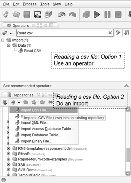
RapidMiner offers at least 20 different operators or ways to connect to your data. The data can be stored in a flat file such as a comma-separated values (CSV) file or spreadsheet, the data can be stored in a database such as a Microsoft Access table, or it can be stored in other proprietary formats such as SAS or Stata or SPSS, etc. If your data is in a database, you need to have at least a basic understanding of databases, database connections and queries in order to use the operator properly. You may choose to simply connect to your data (which is stored in a specific location on disk) or you may choose to import the data set into your local RapidMiner repository itself so that it becomes available for any process within your repository and every time you open RapidMiner, this data set is available for retrieval. Either way, RapidMiner offers easy-to-follow wizards that will guide you through the steps. As you can see in Figure 13.7, when you choose to simply connect to data in a CSV file on disk using a Read CSV operator, you will drag and drop the operator to the main process window. Then you need to configure the Read CSV operator by clicking on the Import Configuration Wizard, which will lead you through a sequence of steps to read the data in.2 The search box at the top of the operator window is also very useful—if one knows even part of the operator name then it’s easy to find out if RapidMiner provides such an operator. For example, to see if there is an operator to handle CSV files, type “CSV” in the search field and both Read and Write will show up. Clear the search by hitting the red X. Using search is a quick way to navigate to the operators if you know some part of their name. Similarly try “principal” and you see the operator for principal component analysis even though you might not know where to look initially. Also, this search shows you the hierarchy of where the operators exist, which helps one learn where they are.

On the other hand, if you choose to import the data into your local RapidMiner repository, you can click on the green down arrow in the Repositories tab (as shown in Figure 13.7) and select Import CSV File. You will immediately be presented with the same five-step data import wizard. In either case, the data import wizard consists of the following steps:
1. Select the file on the disk that should be read or imported.
2. Specify how the file should be parsed and how the columns are delimited. If your data has a comma “,” as the column separator in the configuration parameters, be sure to select it. By default, RapidMiner assumes that a “;” (semicolon) is the separator.
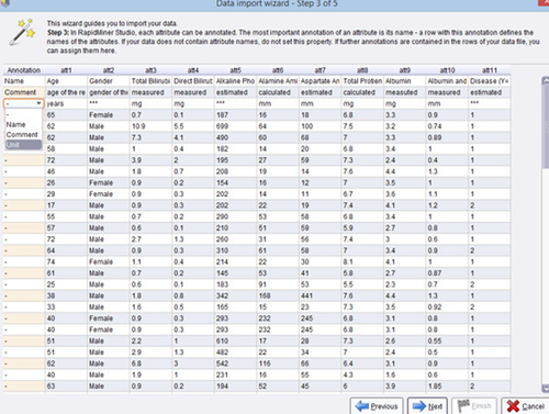
3. Annotate the attributes by indicating if the first row of your data set contains attribute names (which is usually the case). If you data set has first row names, then RapidMiner will automatically indicate this as “Name. If the first few rows of your data set has text or information, you will have to indicate that for each of the example rows. The available annotation choices are “Name,” “Comment,” and “Unit.” See the example in Figure 13.8.
4. In this step we can change the data type of any of the imported attributes and identify whether each column or attribute are “regular” attributes or special ones. By default, RapidMiner autodetects the data types in each column. However, sometimes we may need to override this and indicate if a particular column is of a different data type. The special attributes are columns that are used for identification (e.g., patient ID or employee ID or transaction ID) only or attributes that are to be predicted. These are called “label” attributes in RapidMiner terminology.
5. In this last step, if you are connecting to the data on disk using Read CSV, you simply hit Finish and you are done (Figure 13.9). If you are importing the data into a RapidMiner repository (using Import CSV File), you will be asked to specify the location in the repository for this.

13.3. Data Visualization Tools
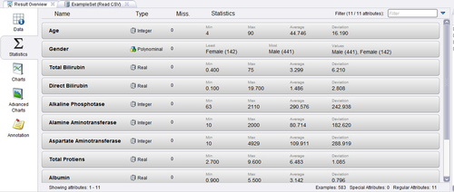
Once you read a data set into RapidMiner, the next step is to explore the data set visually using a variety of tools. Before we jump into visualization, however, it is a good idea to check the metadata of the imported data to verify if we managed to get all the correct information. When the simple process described in Section 13.2 is run (be sure to connect the output of the read operator to the “res”ult connector of the process), we will get an output posted to the Results perspective of RapidMiner. You can see the data table to verify that indeed the data has been correctly imported under the Data tab on the left (see Figure 13.10).
By clicking on the Statistics tab (see Figure 13.11), we can examine the type, missing values, and basic statistics for all the imported data set attributes. Together the data and statistics tabs can tell us that there are 583 samples, 10 regular attributes, and 1 special attribute (the label that was selected in step 4 of the previous section). We can also identify the data type of each attribute (integer, real, or binomial), and some basic statistics. This high-level overview is a good way to ensure that your data set has been loaded correctly and you can now attempt to explore the data in more detail using the visualization tools described below.
There are a variety of visualization tools available for univariate (one attribute), bivariate (two attributes), and multivariate analysis. Select the Charts tab in the Results perspective to access any of the visualization tools or plotter. General details about visualization are available in Chapter 3 Data Exploration.
13.3.1. Univariate Plots
▪ Histogram: A density estimation for numeric plots and a counter for categorical ones.
▪ Quartile (Box and Whisker): Shows the mean value, median, standard deviation, some percentiles, and any outliers for each attribute.
▪ Series (or Line): Usually best used for time series data.
13.3.2. Bivariate Plots
All 2D and 3D charts show dependencies between tuples (pairs, triads) of variables.3
▪ Scatter: The simplest of all 2D charts, which shows how one variable changes with respect to another. RapidMiner allows the use of color; you can color the points to add a third dimension to the visualization.
▪ Scatter Multiple: Allows you to fix one axis to one variable while cycling through the other attributes.
▪ Scatter Matrix: Lets you look at all possible pairings between attributes. Color as usual adds a third dimension. Be careful with this plotter because as the number of attributes increase, rendering all the charts can slow down processing.

▪ Density: Similar to a 2D scatter chart, except the background may be filled in with a color gradient corresponding to one of the attributes.
▪ SOM: Stands for a self-organizing map. It reduces the number of dimensions to two by applying transformations. Points that are “similar” along many attributes will be placed close together. It is basically a clustering visualization method. More details are in Chapter 8 on clustering. Note that SOM (and many of the parameterized reports) does not run automatically so if you switch to that report you will see a blank screen until the inputs are set and the in the case of SOM the “calculate” button is pushed.
13.3.3. Multivariate Plots
▪ Parallel: Uses one vertical axis for each attribute, thus there are as many vertical axes as there are attributes. Each row is displayed as a line in the chart. Local normalization is useful to understand the variance in each variable. However, a deviation plot works better for this.
▪ Deviation: Same as parallel, but displays mean values and standard deviations.
▪ Scatter 3D: Very similar to the scatter 2D chart but allows a three-dimensional visualization of three attributes (four, if you include the color of the points)
▪ Surface: A surface plot is a 3D version of an area plot where the background is filled in.
These are not the only available plotters. Some additional ones are not described here such as pie, bar, ring, block charts, etc. Generating any of the plots using the GUI is pretty much self-explanatory. The only words of caution are that when you have a large data set, generating some of the graphics intensive multivariate plots can be quite time consuming depending upon the available RAM and processor speed.
13.4. Data Transformation Tools
Many times the raw data is in a form that is not ideal for applying standard machine learning algorithms. For example, suppose you have categorical attributes such as gender, and you want to predict purchase amounts based on (among several other attributes) the gender. In this case you want to convert the categorical (or nominal) attributes into numeric ones by a process called “dichotomization.” In the example above, we introduce two new variables called Gender=Male and Gender=Female, which can take (numeric) values of 0 or 1.
In other cases, you may have numeric data but your algorithm can only handle categorical or nominal attributes. A good example is where the label variable being numeric (such as the market price of a home in the Boston Housing example set discussed in Chapter 6 on regression) and you want to use logistic regression to predict if the price will be higher or lower than a certain threshold. Here we want to convert a numeric attribute into a binomial one.
In either of these cases, we may need to transform underlying data types into some other types. This activity is a very common data preparation step. The four most common data type conversion operators are the following:
▪ Numerical to Binominal: The Numerical to Binominal operator changes the type of numeric attributes to a binary type. Binominal attributes can have only two possible values: true or false. If the value of an attribute is between a specified minimal and maximal value, it becomes false; otherwise it is true. In the case of the market price example, our threshold market price is $30,000. Then all prices from $0 to $30,000 will be mapped to false and any price above $30,000 is mapped to true.
▪ Nominal to Binominal: Here if a nominal attribute with the name “Outlook” and possible nominal values “sunny,” “overcast,” and “rain’“is transformed, the result is a set of three binominal attributes, “Outlook = sunny,” “Outlook = overcast,” and “Outlook = rain” whose possible values can be true or false. Examples (or rows) of the original data set where the Outlook attribute had values equal to sunny, will, in the transformed example set, have the value of the attribute Outlook = sunny set to true, while the value of the Outlook = overcast and Outlook = rain attributes will be false.
▪ Nominal to Numerical: This works exactly like the Nominal to Binominal operator if you use the “Dummy coding” option, except that instead of true/false values, we will see 0/1 (binary values). If you use “unique integers” option, each of the nominal values will get assigned a unique integer from 0 and up. For example, if Outlook was sunny, then “sunny” gets replaced by the value 1, “rain” may get replaced by 2, and “overcast” may get replaced by 0.
▪ Numerical to Polynominal: Finally, this operator simply changes the type (and internal representation) of selected attributes, i.e., every new numeric value is considered to be another possible value for the polynominal attribute. In the golf example, the Temperature attribute has 12 unique values ranging from 64 to 85. Each value is considered a unique nominal value. As numeric attributes can have a huge number of different values even in a small range, converting such a numeric attribute to polynominal form will generate a huge number of possible values for the new attribute. A more sophisticated transformation method uses the discretization operator, which is discussed next.
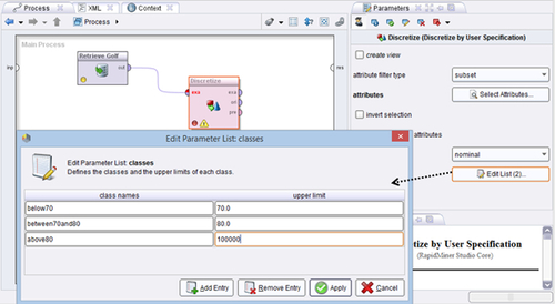
▪ Discretization: When converting numeric attributes to polynominal, it is best to specify how to set up the discretization to avoid the previously mentioned problem of generating a huge number of possible values—you do not want each numeric value to appear as an unique nominal one, but rather have them binned into some intervals. We can discretize the Temperature in the golf example by several methods: we can discretize using equal-sized bins with the Discretize by Binning operator. If we select two bins (default) we will have two equal ranges: [below 74.5] and [above 74.5], where 74.5 is the average value of 64 and 85. Based on the actual Temperature value, the example will be assigned into one of the two bins. We can instead specify the number of rows falling into each bin (Discretize by Size operator) rather than equal bin ranges. We can also discretize by bins of equal number of occurrences by choosing to Discretize by Frequency, for example. Probably the most useful option is to Discretize by User Specification. Here we can explicitly provide ranges for breaking down a continuous numeric attribute into several distinct categories or nominal values using the table shown in Figure 13.12a. The output of the operator performing that discretization is shown in Figure 13.12b.
Sometimes we may need to transform the structure of an example set or “rotate it” about one of the attributes, a process commonly known as “pivoting” or creating pivot tables. Here is a simple example of why we would need to do this operation. The table consists of three attributes: a customer ID, a product ID and a numeric measure called Consumer Price Index (CPI) (see Figure 13.13a). We see that this simple example has 10 unique customers and 2 unique product IDs. What we would like to do is to rearrange the data set so that we have two columns corresponding to the two product IDs and aggregate4 or group the CPI data by customer IDs. This is because we would like to analyze data on the customer level, which means that each row has to represent one customer and all customer features have to be encoded as attribute values.
This is accomplished simply with the Pivot operator. We select “customer id” as the group attribute and “product id” as the index attribute as shown in Figure 13.13b. If you are familiar with Microsoft Excel’s pivot tables, the group attribute parameter is similar to “row label” and the index attribute is akin to “column label.” The result of the pivot operation is shown in Figure 13.13c.
A converse of the Pivot operator is the De-pivot operator, which reverses the process described above and may sometimes also be required during our data preparation steps. In general a De-pivot operator converts a pivot table into a relational structure.


In addition to these operators, you may also need to use the Append operator to add examples to an existing data set. Appending an example set with new rows (examples) works as the name sounds—you end up attaching the new rows to the end of the example set. You have to make sure that the examples match the attributes exactly with the main data set. Also useful is the classic Join operator, which combines two example sets with the same observations units but different attributes. The Join operator offers the traditional inner, outer, and left and right join options. An explanation for joins is available in any of the books that deal with SQL programming as well as the RapidMiner help, which also provides example processes. We will not repeat them here.
Some of other common operators we have used in the various chapters of the book (and are explained there in context) are:
▪ Rename attributes
▪ Select attributes
▪ Filter examples
▪ Add attributes
▪ Attribute weighting
13.5. Sampling and Missing Value Tools
Data sampling might seem out of place in today’s big data–charged environments. Why bother to sample when we can collect and analyze all the data we can? Sampling is a perhaps a vestige of the statistical era when data was costly to acquire and computational effort was costlier still. However there are many situations today with almost limitless computing capability, where “targeted” sampling is of use. A typical scenario is when building models on data where some class representations are very, very low. Consider the case of fraud prediction. Depending upon the industry, fraudulent examples range from less than 1% of all the data collected to about 2 to 3%. When we build classification models using such data, our models tend to be biased and would not be able to detect fraud in a majority of the cases with new unseen data, literally because they have not “learned” well enough!
Such situations call for “balancing” data sets where we need to sample our training data and increase the proportion of the minority class so that our models can be trained better. The plot in Figure 13.14 shows an example of imbalanced data: the “positive” class indicated by a circle is disproportionately higher than the “negative” class indicated by a cross.
Let us explore this using a simple example. The data set shown in the process in Figure 13.15 is available in RapidMiner’s Samples repository and is called “Weighting.” This is a balanced data set consisting of about 500 examples with the label variable consisting of roughly 50% “positive” and 50% “negative” classes. Thus it is a balanced data set. When we train a decision tree to classify this data, we get an overall accuracy of 84%. The main thing to note here is that the decision tree recall on both the classes is roughly the same: ∼86% as seen in Figure 13.15.
We now introduce a subprocess called “Unbalance,” which will resample the original data to introduce a skew: the resulting data set has more “positive” class examples than “negative” class examples. Specifically, we now have a data set with 92% belonging to the positive class (92% class recall) and 8% belonging to negative class (8% class recall). The process and the results are shown in Figure 13.16. So how do we address this data imbalance?

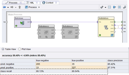

There are several ways to fix this situation. The most commonly used method is to resample the data to restore the balance. This involves undersampling the more frequent class—in our case, the “positive” class—and oversampling the less frequent “negative” class. The “rebalance” subprocess achieves this in our final RapidMiner process. As seen in Figure 13.17, the overall accuracy is now back to the level of the original balanced data. The decision tree also looks a little bit similar to the original, whereas for the unbalanced dataset it was reduced to a stub. An additional check to ensure that accuracy is not compromised by unbalanced data is to replace the accuracy by what is called “balanced accuracy.” It is defined as the arithmetic mean of the class recall accuracies, which represent the accuracy obtained on positive and negative examples, respectively. If the decision tree performs equally well on either class, this term reduces to the standard accuracy (i.e., the number of correct predictions divided by the total number of predictions).

There are several built-in RapidMiner processes to perform sampling: Sample, Sample (Bootstrapping), Sample (stratified), Sample (Model-Based), and Sample (Kennard-Stone). Specific details about these techniques are well described in the software help. We want to only remark on the Bootstrapping method here because it is a very common sampling technique. Bootstrapping works by sampling repeatedly within a base data set with replacement. So when you use this operator to generate new samples, you may see repeated or nonunique examples. You have the option of specifying an absolute sample size or a relative sample size and RapidMiner will randomly pick examples from your base data set with replacement to build a new bootstrapped example set.
We will close this section with a brief description of missing value handling options available in RapidMiner. The basic operator is called Replace Missing Values. This operator provides several alternative ways to replace missing values: minimum, maximum, average, zero, none, and a user-specified value. There is no median value option. Basically, all missing values in a given column (attribute) are replaced by whatever option is chosen. A better way to treat missing values is to use the Impute Missing Values operator. This operator changes the attribute with missing values to a label or target variable, and trains models to determine the relationship between this label variable and other attributes so that it may then be predicted.
13.6. Optimization Tools5
Recall that in Chapter 5 on decision trees, we were presented with an opportunity to specify parameters to build a decision tree for the credit risk example (Section 4.1.2, step 3) but simply chose to use default values. Similar situations arose when building a support vector machine model (Section 4.6.3) or logistic regression model (Section 5.2.3), where also we chose to simply use the default model parameter values. When we run a model evaluation, the performance of the model is usually an indicator as to whether we chose the right parameter combinations for our model.6 But what if we are not happy with the model accuracy (or its r-squared value)? Can we improve it? How?
RapidMiner provides several unique operators that will allow us to discover and choose the best combination of parameters for pretty much all of the available operators that need parameter specifications. The fundamental principle on which this works is the concept of a “nested” operator. We first encountered a nested operator in Section 4.1.2, step 2—the Split Validation operator. We also described another nested operator in Section 12.5 in the discussion on wrapper-style feature selection methods. The basic idea is to iteratively change the parameters for a learner until some stated performance criteria are met. The Optimize operator performs two tasks: determine what values to set for the selected parameters for each iteration, and determine when to stop the iterations. RapidMiner provides three basic methods to set parameter values: grid search, greedy search, and an evolutionary search (also known as genetic) method. We will not go deep into the workings of each method, but only do a high-level comparison between them and mention when each approach would be applicable.
To demonstrate the working of an optimization process, we will consider a very simple model: a polynomial function (Figure 13.18). Specifically, we have a function y = f(x) = x6 + x3 – 7x2 – 3x +1 and we wish to find the minimum value of y within a given domain of x. This is of course the simplest form of optimization—we want to select an interval of values for x where y is minimum. As seen in the functional plot, we see that for x in [–1.5, 2], we have two minima: a local minimum of y = –4.33 @ x = –1.3 and a global minimum of y = –7.96 @ x = 1.18. We will show how to use RapidMiner to search for these minima using the Optimize operators. As mentioned before, the optimization happens in a nested operator, so we will describe what is placed inside the optimizer first before discussing the optimizer itself.

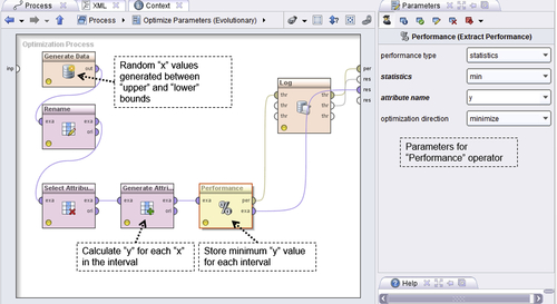
The nested process itself, also called the inner process, is very simple as seen in Figure 13.19a: Generate Data randomly generates values for “x” between an “upper bound” and a “lower bound” (see Figure 13.19b).
Generate Attributes will calculate “y” for each value of “x” in this interval. Performance (Extract Performance) will store the minimum value of “y” within each interval. This operator has to be configured as shown on the right of Figure 13.19a in order to ensure that the correct performance is optimized. In this case, we select “y” as the attribute that has to be minimized. The Rename, Select Attributes, and Log operators are plugged in to keep the process focused on only two variables and to track the progress of optimization.
This nested process can be inserted into any of the available Optimize Parameters operators. Let us describe how we do this with the Optimize Parameters (Grid) operator first. In this exercise, we are basically optimizing the interval [lower bound, upper bound] so that we achieve the objective of minimizing the function y = f(x). As we saw in the function plot, we wish to traverse the entire domain of “x” in small enough interval sizes so that we can catch the exact point at which “y” hits a global minimum.

The grid search optimizer simply moves this interval window across the entire domain and stops the iterations after all the intervals are explored (Figure 13.20). Clearly it is an exhaustive but inefficient search method. To set this process up, we simply insert the inner process inside the outer Optimize Parameters (Grid) operator and select the attributes upper bound and attributes lower bound parameters from the Generate Data operator. To do this, we click on the Edit Parameter Settings option for the optimizer, select Generate Data under the Operators tab of the dialog box, and further select attributes_upper_bound and attributes_lower_bound under the Parameters tab (Figure 13.21).
We will need to provide ranges for the grid search for each of these parameters. In this case we set the lower bound to go from –1.5 to –1 and the upper bound to go from 0 to 1.5 in steps of 10. So the first interval (or window) will be x = [–1.5, 0], the second one will be [–1.45, 0] and so on until the last window, which will be [–1, 1.5] for a total of 121 iterations. The Optimize Performance (Grid) search will evaluate “y” for each of these windows, and store the minimum “y” in each iteration. The iterations will only stop after all 121 intervals are evaluated, but the final output will indicate the window that resulted in the smallest minimum “y.” The plot in Figure 13.22 shows the progress of the iterations. Each point in the chart corresponds to the lowest value of y evaluated by the expression within a given interval. We find the local minimum of y = –4.33 @ x = –1.3 at the very first iteration. This corresponds to the window [–1.5, 0]. If the grid had not spanned the entire domain [−1.5, 1.5], the optimizer would have reported the local minimum as the best performance. This is one of the main disadvantages of a grid search method.


The other disadvantage is the number of redundant iterations. Looking at the plot above, we see that the global minimum was reached by about the 90th iteration. In fact for iteration 90, yminimum = –7.962, whereas the final reported lowest yminimum was –7.969 (iteration 113), which is only about 0.09% better. Depending upon our tolerances, we could have terminated the computations earlier. But a grid search does not allow early terminations and we end up with nearly 30 extra iterations. Clearly as the number of optimization parameters increase, this ends up being a significant cost.
We next apply the Optimize Parameters (Quadratic) operator to our inner process. Quadratic search is based on a “greedy” search methodology. A greedy methodology is an optimization algorithm that makes a locally optimal decision at each step (Ahuja, 2000; Bahmani, 2013). While the decision may be locally optimal at the current step, it may not necessarily be the best for all future steps. k-nearest neighbor is one good example of a greedy algorithm. In theory, greedy algorithms will only yield local optima, but in special cases, they can also find globally optimal solutions. Greedy algorithms are best suited to find approximate solutions to difficult problems. This is because they are less computationally intense and tend to operate over a large data set quickly. Greedy algorithms are by nature typically biased toward coverage of large number of cases or a quick payback in the objective function.
In our case, the performance of the quadratic optimizer is marginally worse than a grid search requiring about 100 shots to hit the global minimum (compared to 90 for a grid), as seen in Figure 13.23. It also seems to suffer from some of the same problems we encountered in grid search.
We will finally employ the last available option: Optimize Parameters (Evolutionary). Evolutionary (or genetic) algorithms are often more appropriate than a grid search or a greedy search and lead to better results, This is because they cover a wider variety of the search space through mutation and can iterate onto good minima through cross-over of successful models based upon the success criteria. As we can see in the progress of iterations in Figure 13.24, we hit the global optimum without getting stuck initially at a local minimum—you can see that right from the first few iterations we have approached the neighborhood of the lowest point. The evolutionary method is particularly useful if we do not initially know the domain of the functions, unlike in this case where we did know. We see that it takes far fewer steps to get to the global minimum with a high degree of confidence—about 18 iterations as opposed to 90 or 100. Key concepts to understanding this algorithm are mutation and cross-over, both of which are possible to control using the RapidMiner GUI. More technical details of how the algorithm works are beyond the scope of this book and you can refer to some excellent resources listed at the end of this chapter (Weise, 2009).


To summarize, there are three optimization algorithms available in RapidMiner all of which are nested operators. The best application of optimization is for the selection of modeling parameters, for example, split size, leaf size, or splitting criteria in a decision tree model. We build our machine learning process as usual and insert this process or “nest” it inside of the optimizer. By using the Edit Parameter Settings … control button, we can select the parameters of any of the inner process operators (for example a Decision Tree or W-Logistic or SVM) and define ranges to sweep. Grid search is an exhaustive search process for finding the right settings, but is expensive and cannot guarantee a global optimum. Evolutionary algorithms are very flexible and fast and are usually the best choice for optimizing machine learning models in RapidMiner.
Conclusion
As with other chapters in this book, the RapidMiner process explained and developed in this discussion can be accessed from the companion site of the book at www.LearnPredictiveAnalytics.com. The RapidMiner process (∗.rmp files) can be downloaded to the computer and can be imported to RapidMiner from File > Import Process. The data files can be imported from File > Import Data.
This chapter provided a 30,000-foot view of the main tools that one would need to become familiar with in building predictive analytics models using RapidMiner. We started out by introducing the basic graphical user interface for the program. We then discussed options by which data can be brought into and exported out of RapidMiner. We provided an overview of the data visualization methods that are available within the tool, because quite naturally, the next step of any data mining process after ingesting the data is to understand in a descriptive sense the nature of the data. We then introduced tools that would allow us to transform and reshape the data by changing the type of the incoming data and restructuring them in different tabular forms to make subsequent analysis easier. We also introduced tools that would allow us to resample available data and account for any missing values. Once you are familiar with these essential data preparation options, you are in a position to apply any of the appropriate algorithms described in the earlier chapters for analysis. Finally, in Section 13.6 we introduced optimization operators that allow us to fine-tune our machine learning algorithms so that we can develop an optimized and good quality model to extract the insights we are looking for.
With this high-level overview, one can go back to any of the earlier chapters to learn about a specific technique and understand how to use RapidMiner to build models using that machine learning algorithm.
..................Content has been hidden....................
You can't read the all page of ebook, please click here login for view all page.