
Chapter 12
Risk-Neutral Pricing in the (B, S) Economy: One Underlying Stock
At this point we have the necessary tools in stochastic analysis for developing the theory of derivative pricing and hedging in continuous time in an economy where risky assets are modelled as Itô processes. In this chapter we consider an economy with two securities: a single tradable risky asset, namely, a stock, and a money market (bank) account or a bond. We refer to this as a (B, S) economy with only two tradable assets: B stands for the bank account or bond and S stands for the stock. More specifically, this chapter is devoted to presenting the theoretical framework solely within the classical case of an economy where the interest rate is fixed and the stock price is modelled as a standard geometric Brownian motion (GBM) with constant growth rate and constant volatility. The case in which the stock pays a dividend yield is also included later. The only source of randomness driving the stock price is a single Brownian motion. This is also referred to as the standard Black–Scholes framework. This can be thought of as the continuous-time analogue of the standard binomial tree model which was formally discussed in great detail in Chapter 7. The analogues of the up and down market moves in discrete time are now random movements of the underlying (driving) Brownian motion. The same important underlying concepts of self-financing, replication, hedging, arbitrage, and no-arbitrage pricing of derivative contracts in discrete time now carry over into the continuous-time setting.
All appropriately discounted tradable assets are martingales under an equivalent martingale (risk-neutral) measure. In particular, by using a self-financing replication strategy, we will arrive at the risk-neutral pricing formula that expresses the current price of any attainable European-style derivative, including contracts with path-dependent payoffs, as a conditional expectation (under the risk-neutral or equivalent martingale measure) of the discounted payoff. The class of derivative securities that are attainable is quite general. This chapter also includes a discussion of this and its relation to hedging and pricing. When pricing a non-path-dependent European-style derivative, the inherent Markov property reduces the risk-neutral pricing formula to a conditional expectation where the (discounted) Feynman-Kac formula allows us to arrive at the infamous Black–Scholes–Merton PDE for the current price of the derivative (option) contract. Recall that in Chapter 11 we made the important connection between the SDE of an Itô process, the (discounted) conditional expectation of a (payoff) function of the terminal value of the process, and the corresponding terminal (or initial) value PDE problem. This is the essence of the Feynman–Kac representation. Our discussion on the theoretical framework of the (B, S) economy culminates in the risk-neutral pricing formulation. We then apply this formulation to derivative pricing problems, where we explicitly derive pricing and hedging formulae for various European contracts, such as standard calls and puts, as well as more complex options such as compound options. We finally also apply the risk-neutral pricing formulation to path-dependent derivatives such as barrier options and lookback options.
12.1 Replication (Hedging) and Derivative Pricing in the Simplest Black–Scholes Economy
Following Section 11.8 of Chapter 11, we fix a filtered probability space (Ω, ℱ, ℙ, ), where is a filtration for standard Brownian motion, i.e., {W(t)}t≥0 is a standard (ℙ, )-BM where ℙ is the physical (real-world) measure. The first base security, B, in this market is the bank account whose price process is denoted by {B(t)}0≤t≤T. In this section we assume a constant interest rate r where B(t) = ert, i.e., B(0) = 1 and B(t) is one unit (dollar) of investment compounded continuously with fixed rate r over time [0, t]. The second base security is the stock whose price process is assumed to be a standard GBM satisfying the SDE
with constant drift µ and constant volatility σ > 0. We recall Example 11.15 in Section 11.8 of Chapter 11. There we showed, by a simple application of Girsanov’s Theorem, that there is a unique risk-neutral measure , defined by (11.96), where is a standard -BM. The discounted stock price process is a -martingale. For convenience, we repeat some of the important equations here. In particular, the stock satisfies the SDE
with solution
The discounted stock price process, with discount factor D(t) := 1/B(t) = e−rt, is a -martingale:
Note also that dB(t) = rB(t)dt has an identically zero coefficient in and that is trivially a (constant) martingale under any measure. Hence, is an equivalent martingale measure (EMM) with the bank account as a numéraire asset.
As in the discrete-time models, we assume no arbitrage in the market and will, below, set up a self-financing replicating portfolio strategy in the two base securities such that the value of the portfolio replicates the value of the financial derivative at some future (maturity) time T. In the absence of arbitrage, the time-t value of the self-financing replicating portfolio must therefore equal the no-arbitrage price of the derivative. Let {Vt}0≤t≤T denote the price process of the derivative security where Vt is the price of the derivative at time t ≤ T. At maturity T, the derivative price is given by the payoff value VT, which is an ℱT-measurable random variable. In the present model, VT is generally some functional of the Brownian motion (BM) up to time T or equivalently some functional of the underlying stock price process {S(t)}0≤t≤T. This functional can be quite complex for a general path-dependent payoff, although for a non-path-dependent derivative (as, for example, a standard call or put) the payoff is only a function of the terminal stock value S(T).
In this (B, S) economy any portfolio (trading) strategy is a continuous sequence of portfolios in the two base assets: (βt, Δt), 0 ≤ t ≤ T, with each process {βt}0≤t≤T and {Δt}0≤t≤T assumed to be adapted to the filtration . As in the binomial model, βt represents the time-t position in the bank account where βt < 0 corresponds to a loan and βt > 0 is an investment. The hedge position Δt is the number of shares held in the stock at time t where Δt < 0 corresponds to shorting the stock and Δt > 0 is a long position. Since we are in continuous time, trading (i.e., portfolio re-balancing) is allowed at any moment in time. The investor begins with a given initial wealth Π0, which completely finances the initial portfolio with positions (β0, Δ0) and subsequently trades at every time t ∊ [0, T] while holding Δt shares in the stock and βt units in the bank account, i.e., this is represented by the portfolio value process for t ∊ [0, T]:
In what follows, we will only consider self-financing portfolio strategies. In analogy with the binomial model, a self-financing portfolio strategy is one in which the differential change in portfolio value is due only to differential changes in the prices of the base assets. Essentially this means that the investor holds the positions (βt, Δt) during the infinitesimal time window [t, t + dt). At time t + dt the BM will have changed by a differential amount dW(t), the stock will have changed its share price by a differential amount dS(t), and the investment in the bank account will have either accrued interest (if βt > 0) or will have decreased in value if βt < 0. Formally, a self-financing portfolio strategy is then a portfolio strategy (βt, Δt), 0 ≤ t ≤ T, such that the cumulative gain in portfolio value is given by
with probability one (a.s.). It is more convenient to work with the differential form of (12.5),
From (12.4) we can express the bank account investment (or loan) as βtB(t) = Πt − ΔtS(t) and substituting this into the above differential, where βt dB(t) = rβtB(t)dt, gives
We can recognize this as the differential form of the continuous-time analogue of the wealth equation we encountered in the binomial model.
As in the binomial model, the discounted self-financing portfolio value process, defined by , is a -martingale. This is readily shown by applying the Itô product rule to the process e−rtΠt ≡ D(t)Πt, where dD(t) dΠt = −rD(t)dt dΠt ≡ 0, and using (12.6):
In the last equation line we made use of (12.3). This therefore shows that is a -martingale and that changes in this discounted self-financing portfolio are due only to changes in the discounted stock price. In integral form we have
Note: we are assuming that the above Itô integral is square integrable. This guarantees that the process defined by (12.8) is a -martingale. This technical detail can be verified later once the option price, and hence the delta position, is obtained.
As in the binomial model, we wish to price derivative contracts that can be replicated by a self-financing portfolio strategy. Let us therefore give a definition of this for the above continuous-time model.
A self-financing strategy (βt, Δt), 0 ≤ t ≤ T, is said to replicate the ℱT-measurable payoff VT at maturity T if ΠT = VT (a.s.), i.e., ℙ(ΠT = VT) = 1. We also say that the payoff VT is attainable.
Let us suppose that a self-financing portfolio strategy that replicates the derivative payoff VT exists. Later we give some discussion on this existence. Then, the cost at any time t ≤ T to set up such a strategy, i.e., the portfolio value Πt, must equal the time-t price of the derivative Vt in order for the investor to hedge (at time t) the short position in the derivative security that has the given attainable payoff VT at future time T, and hence avoid arbitrage. Therefore, we set Vt = Πt for all 0 ≤ t ≤ T for any attainable payoff VT.
The key step now is to make use of the -martingale property in (12.8). In particular, we have
and, since Vt = Πt, then . The discounted derivative price process, {D(t)Vt ≡ e−rtVt}0 ≤ t ≤ T , is therefore a -martingale. We can combine the discount factors, where D(T)/D(t) = B(t)/B(T) = e−r(T −t), giving
This is the risk-neutral pricing formula for the above (B, S) model with a constant interest rate. It is the continuous-time analogue of (7.23) for the binomial model in Chapter 7. We remark that (12.9) was derived for the simplest case where the stock is a standard GBM, but in Chapter 13 we will arrive at the same formula for more general continuous-time stock price processes as long as the payoff is attainable and there exists a risk-neutral measure where the discounted stock (base asset) price process is a -martingale. In Chapter 13 we shall also define an arbitrage strategy in the multi-asset continuous-time framework where it is shown that the existence of a risk-neutral measure implies that no arbitrage strategies are possible within the market model.
The formula in (12.9) may seem very simple; however, its practical use rests upon our ability to calculate the expectation of the payoff conditional on the filtration at time t. The payoff is an ℱT-measurable random variable and it can, in some cases, be quite complex, as it may have a complicated dependence on the path of the stock price process. Hence, the conditional expectation can be quite challenging to compute for complex path-dependent payoffs. The main idea is to simplify the ℱt-conditional expectation to an expectation that can be readily computed. In most practical situations the derivative has a payoff structure that is not too complex. In the binomial model, we have already used the risk-neutral pricing framework to value derivatives having commonly encountered payoffs, such as the standard European call and put options as well as path-dependent options such as lookback and Asian options. Our main tools for analytically pricing such options were the Markov property and the Independence Proposition 6.7 or 6.8. For continuous-time models these tools will also be used within the risk-neutral framework. Moreover, we shall also have other tools at our disposal, such as the PDE approach that is a result of the Feyman–Kac theorems.
Let’s now consider the case of a standard (non-path-dependent) European option with payoff VT = Λ(S(T)) as a ℱT-measurable random variable that is a function of only the terminal (maturity time T) value of the stock price. The important simplification that now follows is due to the Markov property where the conditioning on ℱt is replaced with a conditioning on S(t). We remind the reader of our discussions in Section 11.7 on conditional expectations and the Markov property. In particular, recall that a solution to an SDE is a Markov process and hence (11.42) in Theorem 11.5 applies. The time-t derivative value (expressed as a σ(S(t))-measurable random variable) then takes the form
The derivative pricing function, V(t, S), is a function of calendar (actual) time t and the spot1 (ordinary variable) S > 0 and is given by the discounted expectation of the payoff conditional on S(t) = S:
Given the share price for the stock at time t ≤ T, which is the spot S > 0, then (12.11) gives us the no-arbitrage time-t price of a European option having non-path-dependent attainable payoff Λ(S(T)) at maturity T, where Λ : ℝ+ → ℝ is the payoff function.
We can now generally express the pricing function in (12.11) as an integral over the standard normal density n(z) or equivalently as an integral over the risk-neutral transition PDF. This has essentially already been done in Example 11.11 of Chapter 11 where related formulas were derived under measure ℙ with drift µ (instead of with drift r). Using (12.2), the time-T stock price is given in terms of the time-t price and the -BM increment:
Throughout, we conveniently define τ := T − t as the time to maturity and
which is a standard normal random variable, i.e., under measure . Note that is independent of S(t) since is independent of . Combining these facts into (12.11) gives
By changing integration variables in (12.14), i.e., letting , gives the equivalent pricing formula
where denotes the risk-neutral transition PDF of the stock price process in (12.2):
We recall that this is the time-homogeneous log-normal density in y given by (11.79) with drift parameter µ set to the risk-free rate r. Note that when the stock price process is time homogeneous, as in the present case, the pricing formula is a function of the time to maturity τ = T − t and we shall also denote it by ν(τ, S) := V(t, S), i.e., ν(τ, S) := V(T − τ, S).
We see that (12.14) and (12.15) provide two equivalent expectation (integral) approaches for pricing standard European options on a stock. The transition PDF is the fundamental solution to the PDE in (11.72) with the spot value as a backward variable, x ≡ S, linear diffusion coefficient function σ(x) ≡ σ(S) = σS, and linear drift coefficient function µ(x) ≡ µ(S) = rS. The discounted transition PDF, , and hence the pricing function ν = ν(τ, S) in (12.15), satisfies the PDE in the variables (S, τ) (see (11.77) in Chapter 11):
subject to the payoff condition ν(0+, S) = Λ(S), which is an initial condition in the time to maturity τ ↘ 0. This is the Black–Scholes partial differential equation (BSPDE) for the pricing function expressed as function of the spot and time to maturity variables (S, τ). Since , then (12.17) is equivalent to
subject to the payoff condition V(T −, S) = Λ(S), which is a terminal condition in time t ↗ T. This is the usual BSPDE satisfied by the pricing function V = V(t, S) in the variables (t, S). In fact, the BSPDE in (12.18) arises by direct application of the discounted Feynman– Kac Theorem 11.9 to the conditional expectation in (12.11). [Note that Theorem 11.9 is the same when we replace ℙ, E, and W everywhere by , , and , respectively. All this means is that the probability measure is now the risk-neutral measure . Here, we have the dummy variable x ≡ S and the process X(t) ≡ S(t) is GBM with coefficient functions defined by µ(t, S) := rS, σ(t, S) := σS in the SDE (12.1). In particular, for constant interest rate r the pricing function V(t, S) satisfies the PDE (11.64) in the variables t and S, which is the BSPDE in (12.18).]
Let us now turn our attention to the problem of replicating a derivative claim, i.e., the hedging problem in the simple (B, S) model. We first see how this problem is solved in the case of non-path-dependent payoffs where VT = Λ(S(T)) and Vt = V(t, S(t)). By applying the Itô formula with the differential in (12.1) we obtain:
where is the differential generator corresponding to the GBM process with SDE in (12.1). Now using the fact that the pricing function V(t, S) satisfies the BSPDE in (12.18), i.e., for all (t, S), then
for all t ∊ [0, T]. Assuming the square-integrability condition on the integrand of this Itô integral, {e−rtV(t, S(t))}0≤t≤T is a -martingale. For portfolio replication we require Πt = V(t, S(t)), or , for all t ∊ [0, T]. We see from (12.8) that this can be achieved by setting the initial value of the portfolio Π0 = V0 = V(0, S(0)) and by choosing the delta position such that the respective Itô integrals in (12.8) and (12.19) are equal, i.e., the delta hedge is achieved by choosing
Hence, (12.20) gives the time-t (delta) position in the stock required to dynamically replicate the derivative claim in a self-financing portfolio strategy. Clearly, Δt is ℱt-measurable (in fact it is σ(S(t))-measurable) and is given uniquely by the first derivative (w.r.t. the spot variable S) of the pricing function evaluated at S = S(t). Defining the function , then Δ(t, S) gives the time-t position in the stock given the spot value S. Once the pricing function V(t, S) is known (and hence its derivative computed) the self-financing replicating portfolio in (12.4) is given by Δt = Δ(t, S(t)) positions in the stock and βt = e−rt[V(t, S(t)) − S(t)Δ(t, S(t))] units in the bank account, i.e., the value of the bank account portion of the portfolio at time t is V(t, S(t)) − S(t)Δ(t, S(t)).
Consider the general case where VT is any ℱT-measurable payoff (i.e., generally path dependent). Now, we generally have Vt ≠ V(t, S(t)) (i.e., we do not generally have Vt = as a function of t and S(t)) and hence the above BSPDE and Feynman–Kac results are not generally applicable. However, what is important is that the discounted derivative value process {D(t)Vt}0 ≤ t ≤ T is a (, )-martingale. We now show that we can guarantee that VT is attainable if we make two general assumptions on the payoff:
- VT is square integrable, i.e., E[VT2] < ∞.
- VT is ℱTW-measurable.
[Note that these two conditions are already implicit in the above non-path-dependent case.] The discounted price process {D(t)Vt}0 ≤ t ≤ T is then a square-integrable (, )-martingale. We can now make use of Theorem 11.14, in particular Proposition 11.15 of Chapter 11, where we identify M(t) ≡ D(t)Vt and identify the measure , with constant γ(t) = γ ≡ (r − µ)/σ being ℱtW-adapted. This implies2 and hence {D(t)Vt}0 ≤ t ≤ T is a square-integrable -martingale. Hence, there exists an adapted process, we now denote by , such that (note D(0)V0 = V0):
For portfolio replication we require Πt = Vt, for all t ∊ [0, T]. By (12.21) we see that this is achieved by setting Π0 = V0 and by choosing the delta position such that the integrands in (12.8) and (12.21) are equal, i.e., the delta hedge is achieved by setting [note ]
for all t ∊ [0, T]. This solution for Δt exists, for every , since we are assuming that the volatility parameter σ > 0. Note also that the stock price is a GBM with S(0) > 0 and therefore cannot hit zero in any finite time. Of course, implicit in this existence are also the above assumptions on the derivative payoff. Namely, VT must be ℱtW-measurable and this means that we can only guarantee replication of payoffs whose only source of randomness is the BM driving the stock itself.
We have therefore shown that the model can replicate (hedge) any complex arbitrary path-dependent derivatives with a payoff satisfying the above two assumptions. In this sense we can say that the (B, S) model is a complete market model. The formula in (12.22) asserts the existence of a hedging strategy and therefore justifies the use of the risk-neutral pricing formula in (12.9). We remark that generally (12.22) does not give a practical (or explicit) construction of the hedging strategy. However, there are important examples of common payoffs for which we do have an explicit formula for the delta hedge. For example, in the particular case of a non-path-dependent standard European option we already showed that θ(t) is given explicitly in terms of the derivative of the pricing function:
with the delta position given by (12.20).
12.1.1 Pricing Standard European Calls and Puts
We now use the risk-neutral pricing formulation to derive the well-known Black–Scholes– Merton formulae for the prices of a standard call and put option in the simplest (B, S) model of Section 12.1, where the stock price is a GBM with constant volatility σ > 0 and the bank account has constant interest rate r. Here we are assuming a zero dividend on the stock, but the inclusion of a stock dividend is quite simple, as shown later.
Consider a call option with payoff VT ≡ CT = (S(T) − K)+. This is an example of a non-path-dependent option with payoff function Λ(x) := (x − K)+. Let S(t) = S > 0 be the spot price of the stock at time t ≤ T. Since the payoff depends only on the terminal stock price S(T), the (current) time-t price of this call with strike K > 0 can be found by directly evaluating the integral in (12.14) using the identity (A.1) in the Appendix. We leave this as an exercise for the reader. We recall that in Chapter 4 a brute force integration of (12.14) was also used in deriving the time-0 price of the put option with payoff Λ(x) = (K − x)+. Here we carry out the derivation in an explicit manner that is instructive since it clearly displays the use of the conditional expectation approach and the connection between the different random variables and independence. In particular, using (12.11), the time-t price of the call, C(t, S), is the discounted risk-neutral expectation of the payoff at time T > t, conditional on S(t) = S:
with S(T) given by (12.12). Two conditional expectations need to be computed (where the last term has been expressed as a conditional probability). In both cases we use the fact that in (12.13) is independent of S(t) and, by the Independence Proposition 6.7, this allows us to remove the conditioning upon setting S(t) = S. First, let us rewrite the event {S(T) > K} in terms of and S(t) by simply dividing S(T) in (12.12) by S(t), dividing K by S(t), and taking natural logarithms:
where we define
for all x > 0, τ := T − t > 0. We use the above representation for the event and substitute the expression for S(T), given in (12.12), into the first expectation in (12.23), which is now readily computed by setting S(t) = S, using the independence of and S(t), and then applying the identity3 in (A.1) of the Appendix to evaluate the (unconditional) expectation:
The conditional probability in (12.23) now follows quite simply:
Note that this is also obtained directly from the transition CDF, , of the GBM process under measure , where
Substituting (12.25) and (12.26) into (12.23) completes our derivation of the pricing formula for the standard call:
Having priced the call, we can now easily derive the pricing formula for the put price, P(t, S), by recalling the simple symmetry between the call and put payoffs, i.e., a portfolio in one long call and one short put is equivalent to a portfolio in one long forward contract:
Taking discounted risk-neutral expectations on both sides of (12.28) gives
where we recognize the left-hand side as the difference in the time-t price of the call and put, at strike K. The right-hand side is the time-t price of a forward contract with payoff S(T) − K. This is the put-call parity relation that we have already encountered in our primer chapter (Chapter 4) on derivative securities. It is important to note that this relation is valid for quite general models (i.e., beyond the GBM model). The only assumption is that the discounted stock price is a -martingale. Substituting the call price in (12.27) into (12.29) gives the pricing formula for the standard put:
We leave it as an exercise for the reader to show by direct differentiation that the above call and put pricing functions in (12.27) and (12.30) solve the BSPDE. The initial conditions τ ↘ 0 (equivalently t ↗ T) on the above pricing functions are readily shown to be satisfied by working out the limiting forms (see also Example 11.11):
Hence, both limits equal the unit step function centered at S = K. Using both these limits in (12.27) verifies the payoff condition for the call:
By the same steps applied to (12.30), we verify the payoff condition:
The asymptotic values for the call and put pricing functions for small and large spot values are readily obtained. We leave it as an exercise to show, by directly computing the limits, that
and
The financial interpretation of the above limits is clear. In the limit that the time-t stock price (spot S) is very close to zero, it will remain close to zero within a finite time to maturity τ = T − t. This means that the call will certainly expire out of the money (hence is worthless) and the put will expire completely in the money with payoff K and time-t value e−rτ K. In the limit of arbitrarily large spot value, the stock price will remain arbitrarily large, i.e., the put will certainly expire out of the money (hence is worthless) and the call will expire in the money with an arbitrarily large payoff.
12.1.2 Hedging Standard European Calls and Puts
In Chapter 4 we computed the “delta” of a standard call and put by differentiating the pricing functions. Let us denote the delta of the call at calendar time t by and the delta of the put by . Note that Δc and Δp are also functions of (τ, S), since the pricing functions in (12.27) and (12.30) are expressible as functions of (τ, S). We recall a previous method to derive Δc by simply differentiating (12.27) w.r.t. S, where , while using ,
Here we used the following identity with x = S/K (which we leave as a somewhat tedious exercise in algebra for the reader to show):
The above derivation of Δc is correct but perhaps not the most instructive. We now give an alternate derivation of Δc by directly connecting it to the discounted risk-neutral conditional expectation in (12.25). From the risk-neutral pricing formula in (12.14),
We now differentiate w.r.t. S (as a parameter) inside the expectation or inside the integral and use the property . In the integral we have or in the expectation . We can write the steps compactly as follows by differentiating inside the expectation (note: ),
Here we identified the conditional expectation in (12.25).
It is important to note that the delta of a call is strictly positive, i.e., Δc(t, S) > 0 for all t < T, S > 0, since the CDF is strictly positive for all x ∊ ℝ. Hence, according to (12.20), to replicate a call the writer is continuously re-balancing the self-financing portfolio while always maintaining a delta positive (long) position in the stock given by for τ = T − t > 0. In particular, the time-t investment in the stock, given spot S(t) = S, is
Since Πt = C(t, S(t)) = C(t, S), the time-t value of the bank account (cash) portion of the self-financing portfolio is, upon using (12.27),
This quantity is negative for all t < T, S > 0. Hence, the writer of the call is always maintaining a negative position (loan) in the bank account.
The delta position at maturity t = T is given by the limit t ↗ T of the function in (12.34). From (12.31) we see that, in the limit of zero time to maturity, Δc approaches the unit step function with discontinuity at S = K. Moreover, for any fixed τ > 0, we observe that Δc is a strictly increasing function of S with limiting values of zero and unity:
Figure 12.1 contains typical plots of Δc for different values of τ. We clearly see that Δc approaches the unit step function as τ ↘ 0. As τ ↘ 0, (12.34) gives Δc → 0 for S < K, Δc → 1 for S > K, and for S = K. We see that Δc gets progressively steeper for smaller and smaller values of τ and eventually becomes the unit step function. At a time t just before expiry (i.e., τ ≍ 0), if the stock price lies above K, then Δc ≍ 1 and the hedging replicates the positive payoff of the call after paying off the loan in the amount of K (see (12.31) and the above expression for βtB(t)). On the other hand, if the stock price is below K (out of the money), then Δc ≍ 0 and βtB(t) ≍ 0, so the hedge replicates the zero payoff of the call.

Typical plots of the call delta as function of spot for four different values of time to maturity τ.
There are also scenarios where the stock price S(t) just before expiry (t ≍ T) stays very close to the strike K until time T. There is a fairly high probability (which is easily computed) that the stock price will fluctuate between values below K and above K. These are scenarios where the stock is said to be “pinning the strike.” For values of τ close to zero this would mean that the (hedge) position in the stock would have to be re-balanced, in a short time, between a very small long position (Δc ≍ 0) and a large long position where the replicating portfolio is almost all stock (Δc ≍ 1). This re-balancing requires either selling off a large portion of the underlying stock or buying up a large portion of stock so as to maintain the correct hedge. In particular, if the stock price suddenly moves just before expiry from one side of the strike to the other, then the writer or trader must rapidly trade enough of the underlying stock before expiration in order to hedge the loss against such a movement. In the (B, S) theoretical (idealized) model such transactions are assumed to occur instantaneously (as efficiently as is required!) and without any liquidity issues in trading, i.e., all scenarios are, in theory, hedged. In the real world these kinds of scenarios cannot be hedged effectively in time since instantaneous re-balancing is obviously not possible. Moreover, there are transaction fees associated with each trade. The risk associated with options trading whereby the market price of the stock is pinning the strike is referred to as pin risk. Later we consider the pricing of a so-called soft-strike call. This contract differs from the standard call, as its payoff is everywhere differentiable and it has a continuous range of strikes. This type of option avoids the problem of pin risk when delta hedging.
The delta of a put option, Δp, follows trivially by put-call parity,
The delta of a put is therefore strictly negative and is simply related to the call delta by Δp = Δc − 1. A put option is replicated by continuously re-balancing with a delta negative (short) position in the stock given by . Given spot S(t) = S, the time-t value of the stock portion of the replicating portfolio for the put is given by
The self-financing replicating portfolio value for the put is Πt = P(t, S(t)) = P(t, S), so the corresponding time-t investment in the bank account is
In direct contrast to the call, the put is replicated by always maintaining a positive investment in the bank account.
At maturity t = T, Δp(T, S) = Δc(T, S) − 1= H(S − K) − 1. For τ > 0, Δp is a strictly increasing function of S with limiting values:
The above discussion on hedging and pin risk associated with the call also applies in an obviously similar manner to the put with given strike K. We note that for the put delta the corresponding plots of Δp as a function of S are as in Figure 12.1, where the origin of the vertical axis is simply shifted up by unity.
In closing this section we recall that the delta is one among other so-called “Greeks” of an option that are of interest to practitioners such as options traders. Recall that in Section 4.3.4.4 of Chapter 4 we provided some discussion of these quantities. This chapter is focused on risk-neutral pricing and hedging of options. We leave it as an exercise for the reader to derive the corresponding formulas for the gamma, theta, vega, and rho of a standard call and put expressed as a function of S, τ, K, r, σ.
12.1.3 Europeans with Piecewise Linear Payoffs
Equations (12.25) and (12.26) are useful for pricing any European option having a piece-wise linear payoff with possibly a finite (or countable) number of discontinuities. Actually, the standard call and put options are important special cases of such payoffs with no discontinuity and a discontinuity in their first derivatives. Let’s now consider a simple example of a piecewise constant payoff with a single jump discontinuity.
(Asset-or-Nothing Binary Call) Consider an option that pays the holder the value of the underlying share price of the stock if the stock price at expiry is above a given strike K and is otherwise worthless, i.e., the holder gets the asset (stock) or nothing with payoff function
Derive the risk-neutral pricing formula and the hedging position in the stock for the European option with this payoff.
Solution. Observe that the payoff is also the first term in the standard call option. The risk-neutral pricing formula immediately follows from (12.25):
where τ = T − t. The delta hedge is obtained by straightforward differentiation,
Note that the time-t replicating portfolio is always long in the stock with a bank loan in the amount of .
Recall that a cash-or-nothing binary call has payoff Λ(S) = ?{S≥K}. Hence, a standard call struck at K is a portfolio consisting of K short positions in a cash-or-nothing call and one long position in an asset-or-nothing call, both struck at K.
We now consider a derivation of the risk-neutral pricing formula for a European option with arbitrary piecewise linear payoff, assuming the standard GBM model for the stock. As a general form for the payoff we consider the sum of linear functions restricted to any number n ≥ 1 of nonoverlapping intervals:
with any real constants Ai, Bi and where 0 ≤ a1 < b1 ≤ a2 < b2 ≤ ... ≤ an < bn ≤ ∞. This function can account for a number of jump discontinuities (including no discontinuities), piecewise constant payoffs, and piecewise linear payoffs with any combination of positive and negative slopes.
As a concrete example, let n = 1. A call with Λ(S) = (S − K)+ is then given by (12.37) with parameter choice A1 = 1, B1 = −K, a1 = K, b1 = ∞. A cash-or-nothing binary call with Λ(S) = ?{S≥K} obtains with A1 = 0, B1 = 1, a1 = K, b1 = ∞. The payoff of an assetor-nothing call, Λ(S) = S ?{S≥K}, corresponds to A1 = 1, B1 = 0, a1 = K, b1 = ∞. For n = 2, an example is the butterfly spread with strikes K1 < K2 < K3, K2 = (K1 + K3)/2, which is representable as a linear combination of piecewise linear functions with payoff . This corresponds to setting the parameters in (12.37) to A1 = 1, B1 = −K1, a1 = K1, b1 = K2 and A2 = −1, B2 = K3, a2 = K2, b2 = K3.
In order to make use of the conditional expectation identities in (12.25) and (12.26) we write and express the payoff in (12.37) as
Applying the identities in (12.25) and (12.26) and the linearity property of expectations, we arrive at an analytical expression for the risk-neutral pricing formula of a European option with payoff in (12.37):
where τ = T − t and d±(x, τ) functions defined in (12.24). We leave as an exercise the derivation of a general formula for the delta hedging position Δ(t, S) for this option. The pricing formula in (12.38) is applicable to several payoff forms that occur in practice and we leave some as assigned exercises at the end of this chapter.
12.1.4 Power Options
Power options differ from vanilla European options in that the payoff function is not linear but raised to some power in the underlying spot. We now show how to analytically value such options under the GBM model. Typically, the payoff of a power option is a quadratic function of the stock price. The widest possible application of power options is for addressing the nonlinear risk of option sellers. There was proposed a class of soft-strike options which do not have a single fixed strike price but a continuous range of strikes spread over an interval. As was mentioned earlier, such options allow for addressing limitations of a standard delta hedging when the underlying asset is pinning the strike at the expiration of the option.
More generally, the payoff of a power option may involve the terminal stock price raised to some power, e.g., Sα(T) ≡ (S(T))α with either positive or negative exponent α ≠ 0, as well as other terms involving Sα(T) times an indicator function restricting the value of S(T) on some interval. Let’s assume that the payoff is some linear combination of elemental payoffs having any of the three forms
where A1 < A2 and A are nonnegative constants. Hence, by the risk-neutral derivative pricing formulation the present value of a power option at time t < T will involve expectations of the above payoffs under the risk-neutral measure . We can handle all of the above three payoffs by simply deriving a formula for the conditional expectation of the payoff Sα(T) ?{S(T)>A}, for any A ≥ 0, since
Note also that for A1 = 0 we have
where ?{S(T)>0} = 1 since the stock price is always positive. The expectation of Sα(T), conditional on a given spot value S(t) = S > 0, for any t < T, is easily calculated using (12.12) raised to the exponent α. Again we use the fact that in (12.13) is independent of S(t) (under measure ), which allows us to remove the conditioning upon setting S(t) = S:
where τ := T − t. The only difference between the conditional expectation in (12.40) and that of Sα(T) ?{S(T)>A} is the indicator function term. By the exact same step as in our derivation of the standard call and put options, the indicator random variable term simplifies,
with d± defined in (12.24), i.e., . Then, conditioning on S(t) = S and using independence,
The last expectation was computed using the identity in (A.1) of the Appendix and noting that . Note that this formula also recovers (12.40) in the limit A ↘ 0. This follows by monotone convergence of the expectations where ?{S(T)>A} ↗ ?{S(T)>0} = 1, as A ↘ 0. Based on (12.39) and the linearity property of the expectation, using (12.41) for A = A1 and for A = A2 leads to the formula
We now use the formulae in (12.40)–(12.42) to price a soft-strike call option in the following example.
(Soft-Strike Call Option) Consider the soft-strike European call option with payoff function
where the constant a ∊ [0, K] and K is a central strike value.
- (a) Describe the main features of the graph of Λa(S) for all S > 0.
- (b) Assume the stock price process {S(t)}t≥0 is a GBM with constant interest rate r and volatility σ. Let S(t) = S be the spot price of the stock at current time t < T. Derive the no-arbitrage pricing formula for a European-style option with the above payoff function.
Solution.
(a) (see Figure 12.2) Note that Λa(S) ≥ (S − K)+, where Λa(S) ↘ (S − K)+ as a ↘ 0, i.e., as a function of the parameter a, the soft-strike payoff decreases monotonically to the standard call payoff as a ↘ 0. In contrast to the standard call payoff (S − K)+ whose derivative w.r.t. S has a unit jump discontinuity at S = K, the payoff Λa(S) has a continuous derivative for all S. The left and right derivatives at S = K − a are the same, Λ′a (K − a) = 0, and the left and right derivatives at S = K + a are the same, Λ′a (K + a) = 1. Combining this with the derivative for S ∊ (K − a, K + a), the payoff has a continuous derivative w.r.t. S given by
Moreover, the payoff has a piecewise constant second derivative Λ′a(S). In fact, the payoff can be expressed as an integral over the standard call payoff function (S − k)+ by employing a continuum of strikes k ∊ (K − a, K + a) (see Exercise 12.14).
(b) Express Λa(S(T)) as a linear combination of payoffs involving the different powers of S(T) multiplying indicator random variables:
The option value at current time t is then the discounted conditional expectation of this payoff. Let V(t, S) ≡ C(t, S; K, a) denote the time-t value of the soft-strike call where we include the dependence on the parameters a, K defining the payoff. By linearity of expectations:
We now use the formulas given in (12.41) and (12.42) for respective powers of α =1, 2, as well as our previously derived formulas for the risk-neutral conditional probability that S(T) lies above a strike level or within an interval. Combining all terms gives
where τ = T − t is the time to maturity and d±(x, τ) are defined in (12.24).

Based on the pricing formula in (12.45) we can compute the delta hedging position in the stock. Moreover, we can readily price the corresponding soft-strike put option with given center strike K and width a. We leave this as an exercise for the reader (see Exercise 12.15). There are also other power options that are readily priced with the use of the formulae in (12.40)–(12.42) and these are assigned as exercises at the end of this chapter.
12.1.5 Dividend Paying Stock
12.1.5.1 The Case of Continuous Dividend Paying Stock
Let us now consider the above (B, S) model where the stock is a standard GBM which also pays a dividend with a constant continuous yield q > 0 per unit of time. During an infinitesimal time dt the holder of the stock receives a dividend payment of qS(t)dt that is in proportion to the stock price at time t. We can see this from the return due only to the dividend, for small time interval δt ≍ 0. By no-arbitrage this dividend payment to the stock holder must be exactly balanced by a decrease in the share price of the stock. Hence, in the physical P-measure there is the additional negative drift term, −qS(t)dt, due to the dividend. The stock price process is a GBM with SDE
By the same unique risk-neutral measure as above, where is a standard -BM, the above SDE takes the form
For a nonzero dividend, the risk-neutral drift of the stock price is (r − q) in the place of r. Given an arbitrary initial stock value S(0) > 0, this SDE has a unique solution
The time-T stock price is given in terms of the time-t price and a -BM increment:
Note that the process acts as a nondividend stock, i.e., it has the same risk-neutral drift, r, as any non-dividend-paying asset. Discounting the price process with the bank account gives as a -martingale.
The replicating portfolio is the same as given in (12.4). The portfolio is invested in the amount of ΔtS(t) in the stock, so the dividend payment is qΔtS(t)dt over time dt. This term is now added to the differential change in the self-financing portfolio in (12.6), giving
In the last line we used (12.46). This is of the same form as in (12.7) and hence (12.8) still holds where the discounted self-financing portfolio value process is a -martingale. The risk-neutral pricing formula in (12.9) as well as (12.10) and (12.11) still hold. The conditions and arguments given in Section 12.1 that guarantee that a claim can be replicated (hedged) are the same as in the case of zero dividend on the stock.
The only difference is that the stock has drift parameter (r − q) instead of r, i.e., S(t) is given by (12.47) instead of (12.2) and (12.48) replaces (12.12). So the question is, in terms of pricing, what does this change? The general answer is actually very simple given the solution in the case that q = 0. Let’s take a look at how (12.14)–(12.20) change. Using (12.48) in the place of (12.12), the expectations in (12.14) and (12.15) now become
where is now the risk-neutral transition PDF of the stock price GBM process with drift r − q, i.e., with r replaced by r − q in (12.16). The generator for the stock price process with SDE in (12.46) is defined by . Hence, the respective Black–Scholes partial differential equations in (12.17) and (12.18) are now
subject to ν(0, S) = Λ(S) and
subject to V(T, S) = Λ(S). Note that the dividend only changes the drift term where has been replaced by . Everything else is the same, including the discount factor. Equations (12.19) and (12.20) are then also the same, i.e., the delta hedge position is the same. Of course, the derivative value V(t, S) for q ≠ 0 differs from the value when q = 0.
We now show that the derivative pricing formula for q ≠ 0 (nonzero stock dividend) obtains trivially from the corresponding pricing formula for q = 0 (zero dividend), given arbitrary payoff VT = Λ(S(T)). To precisely describe this, let V(t, S; r, q) be the time-t price of the derivative for given interest rate r and stock dividend q. This function has a dependence on parameters r and q, as well as other parameters that we simply suppress. The corresponding price when q = 0 is then V(t, S; r, 0). The function V(t, S; r, q) is given by (12.50) and V(t, S; r, 0) is given by (12.14). Multiplying out the discount factor in both cases gives erτ V(t, S; r, q) = [erτ V(t, S; r, 0)]|r→r− q, which is equivalent to
From this relation we see that the pricing function (on the left) for q ≠ 0 is given by the corresponding pricing function (on the right) for q = 0 after replacing the interest rate r by r − q and multiplying the function by e−qτ , τ = T − t. The simple example below shows how (12.53) is very easily applied to a standard call and put.
Apply the symmetry in (12.53) to (12.27) and obtain pricing formulae for the standard European call for a stock with continuous constant dividend yield q.
Solution. Let C(t, S; r, q) ≡ C(τ, S, K, σ, r, q) denote the pricing formula for the call with stock dividend q. For q = 0, C(t, S; r, 0) ≡ C(τ, S, K, σ, r, 0) is given by (12.27):
Applying (12.53), C(t, S; r, q) = e−qτ C(t, S; r − q, 0) = e−qτ C(τ, S, K, σ, r − q, 0):
where τ = T − t and d±(x, τ) are defined in (12.24).
This example also points out another very useful simple symmetry where the standard option pricing function, for given dividend q, is given by the original (zero dividend) pricing function with spot value S replaced by the “effective spot” value e−qτ S (keeping everything else the same). This is an alternatively useful symmetry that we can apply to immediately obtain the pricing formula for q ≠ 0 by substituting e−qτ S for S within the pricing formula for q = 0. We can express this additional symmetry as
We see quite trivially how this symmetry works in the above example of the call where setting e−qτ S for S in (12.27) gives (12.54). Applying either (12.53) or (12.55) to (12.30) gives the corresponding pricing formula for the put option on a dividend paying stock,
The put-call parity relation in (12.29) now takes the more general form,
where we simply write C(t, S) = C(t, S; r, q) and P(t, S) = P(t, S; r, q).
Corresponding symmetry relations for the delta hedging position also follow. Let us denote . Then,
By the chain rule, differentiating (12.55) gives us an alternative symmetry:
For example, consider a call where (12.34) gives Δc(t, S; r, 0) and by either (12.58) or (12.59):
We point out that this formula can also be obtained using our previous derivations, i.e., without use of the symmetry relation in (12.58).
If we assume no knowledge of the above symmetry and no prior pricing formula for q = 0, then we can of course derive the pricing formula in (12.54) from first principle, by employing the same steps that lead to (12.27) where we had q = 0. Namely, we substitute the expression for S(T) in (12.48) into the discounted expectation in (12.23) and evaluate by using the identities in (12.25) and (12.26) where now the drift r − q replaces r, i.e., (12.25) and (12.26) become
and
Combining these into (12.23) gives the call pricing formula in (12.54). Using similar steps, or by put-call parity, we obtain the above put pricing formula. The pricing formulae for European derivatives on a dividend paying stock for all other types of payoffs, including those we considered in Sections 12.1.3 and 12.1.4, also follow by the above symmetry relation. Alternatively the formulae can be derived from first principles based on the identities in (12.61) and (12.62). In the case of power options on a dividend payoff stock, we have the identities in (12.40), (12.41), and (12.42) where r is replaced by r − q (or equivalently do not replace r but replace S by e−qτ S).
[Technical Remark: We now give a more technical argument showing that the above symmetry relation in (12.53) holds as a particular case of a similar symmetry for more complex path-dependent payoffs. Consider an arbitrary European derivative where the payoff VT has a path dependence on the stock, i.e., is a functional of the stock price process from time t to T. Examples of these derivatives are barrier options, Asian options, lookback options, etc. In general, the derivative price Vt is an ℱt-measurable random variable where (12.9) holds for any attainable claim VT. More specifically, denote by {S(r − q)(u) : t ≤ u ≤ T} the path of the stock price process defined by the risk-neutral drift parameter r − q (and volatility σ) and let Vt = Vt(r, q) be the corresponding derivative price at time t, for any constant interest rate r and constant dividend yield q. Now, let VT depend on any segment of the stock price path, including the entire path history from time t to T. We write this as a functional, VT(r, q) = F{S(r − q)(u) : t ≤ u ≤ T}. Note that VT(r − q, 0) = F {S(r − q − 0)(u) : t ≤ u ≤ T} = VT(r, q). Hence, by (12.9),
So (12.53) is recovered for standard non-path-dependent payoffs with spot S(t) = S giving Vt(r, q) = V(t, S; r, q). However, we note that the relation in (12.55) does not generally hold for path-dependent derivative pricing.]
12.1.5.2 The Case of Discrete-Time Dividends
The continuous-time dividend payment model of a stock in the previous section led to analytical pricing formulae for European derivatives that have the same form as the formulae with zero dividend. We shall mostly adopt this model in further applications. In practice, however, stocks in the market pay dividends at discrete regular intervals of time. Let’s suppose that at present time t0 < T we know the fixed future dividend dates, Ti, i = 1, ... , N, t0 < T1 < ... < TN ≤ T. At each time Ti the dividend payment div(Ti) is a proportion of the stock value at time Ti, i.e., div(Ti) = diS(Ti), where 0 ≤ di ≤ 1 is the dividend percentage. When no dividend is paid at time Ti we have di = 0 and when the full share value of the stock is paid at time Ti then di = 1 and the stock becomes worthless for all time after Ti. Typically, we can assume 0 < di < 1 for i = 1, ..., N. We remark that by writing di = qi (Ti − Ti−1) then qi is a dividend yield (rate) that is fixed within the time interval (Ti−1, Ti].
The model for the stock is then as follows. Between the ith dividend date and just before the (i + 1)th dividend date, i.e., within any time interval between dividend payments, the stock price evolves simply as a GBM according to the SDE in (12.1). Hence the stock price at time t0 ≤ t < T1 is given in terms of the spot S(t0) ≡ S0 as
At time t = T1−:
where we use the notation for i = 1, . . . , N. For times t ∊ [Ti−1, Ti), i = 2, ..., N, we have
and in particular for t = Ti−, just before the ith dividend date,
Finally, for the last interval [TN, T],
Now, at each dividend payment date Ti, i = 1, ..., N, the stock price instantaneously decreases by a fraction di due to the dividend payment. This is expressed as
Hence, substituting the expression for S(Ti−) in (12.64) into this last equation gives the evolution of the stock price from one discrete dividend date to the next as
For time t0 to just after the first dividend payment time T1 we have
Multiplying out the stock price ratios for all adjoining time intervals including the first and last interval (note: this is a telescoping product) gives
where . In the last line we simplified the sum in the exponents where .
From (12.68) we see that the stock price S(T) is a GBM random variable with drift r and volatility σ. The overall discount factor due to all the dividends is multiplying the actual initial stock price S0 giving the initial value now acting as effective initial stock price at time-t0. We recall that in the case of a continuous dividend the quantity e−qτ S0 acts in the place of when pricing a non-path-dependent European derivatives. Hence, all the time-t0 pricing formulae for non-path-dependent (standard) European derivatives on the stock are obtained by using the initial value in the place of S0. This is clear by substituting the time-T stock price expression in (12.68) into the risk-neutral pricing (expectation) formula with (non-path-dependent) payoff VT = Λ(S(T)). In particular, let V(t0, S; d) represent the European pricing formula for the above stock model with discrete dividends, within the time interval (t0, T), grouped in a vector d = (d1, ..., dN). Accordingly, let V(t0, S) ≡ V(t0, S; 0) be the pricing function for zero dividends. Then, the analogue of (12.55) is the relation
The pricing functions for a standard call option, put option, power option, etc., follow immediately based on the formulae for zero dividends. For example, simply setting the spot value to in (12.27) gives the pricing formula for the time-t0 call option with discrete dividends d1, ..., dN within the time to maturity τ = T − t0:
where
12.2 Forward Starting and Compound Options
We are now equipped to readily develop pricing and hedging formulae for other classes of options besides the standard European options considered so far where we assumed a payoff VT = Λ(S(T)). Rather than having a payoff that depends solely on the terminal stock price S(T) at maturity T, there are European-style options that can have stipulations at a finite number of intermediate dates within the lifetime of the option. These types of options are examples of what can be termed multistage options. As in most options, there are simpler and more complex versions of these contracts.
Examples of simpler contracts are forward starting options with one intermediate date T1 < T. The holder enters the contract at a time t < T1 such that at time T1 the contract has the value of an option (say a European call) on an underlying stock which expires at T. Generally we can represent the option value at time T1 as a function of . The time-T payoff, VT = Λ(S(T1), S(T)), of the option can depend upon S(T1) and S(T). By risk-neutral pricing we have (discounting from T back to T1)
Let V(t, S) ≡ V(t, S; T1, T) denote the time-t value of the forward starting option with given spot S(t) = S. By the Markov property of the stock price process, conditioning on ℱt reduces to conditioning on S(t). Applying again the risk-neutral pricing formula (discounting from time T1 to t) and the tower property4 finally gives us the time-t price as a single conditional expectation discounted from T to t:
For instance, in a forward starting call the holder enters the contract at a time t < T1, prior to an intermediate date T1, whose value at time T1 is a call on an underlying stock initiated at the “forward” time T1. The call initiated at time T1 expires at date T > T1 and has some strike specification, which is generally a function of the stock price S(T1) (i.e., the strike is not a constant specified value). Specifically, the forward starting call can be specified as having strike , then Λ(S(T1), S(T)) = (S(T) − S(T1))+. Hence, as viewed at present time t, the strike is a random variable corresponding to the price of the stock at time T1. Inserting the payoff into (12.72) gives the time-t price of this forward starting call
Let’s assume the stock price is a GBM given by (12.2) with zero dividend. The addition of a continuous constant dividend yield q on the stock can be done trivially by applying the symmetry relation in (12.53) to the resulting pricing formula. The above expectation is readily evaluated by writing the payoff as
where random variable is independent of S(T1). Hence, using the tower property in reverse gives a nested expectation with an inner expectation conditional on S(T1) as in (12.72):
Here we pulled S(T1) out of the inner expectation as it is -measurable; then the inner condition is dropped since Y is independent of S(T1), and finally the unconditional expectation is a constant that is factored out of the expectation conditional on S(t) = S. Note that we have also factored the discount term into two parts. The first term on the right in (12.73) is recognized as the Black–Scholes price of a call with no dividend, time to maturity T − T1, effective strike and spot of unity:
where
The second term in (12.73) gives the spot S since . Multiplying the expression in (12.74) by S produces the pricing formula:
We observe that this pricing function is linear in the spot S since the term in square brackets depends only on parameters r, σ, T1,T . The delta hedge is then trivially given by the term in brackets, . This is a constant hedge position having no dependence on time t and spot S. What is then interesting is that this forward starting call can be hedged statically in time! Other related forward starting option problems are left as exercises for the reader (see Exercises 12.19 and 12.20).
We now consider the problem of pricing a more complex class of options known as compound options. As the name implies, such contracts are options on options. Here we shall assume the simplest types of compound options that involve an (outer) option to buy or sell another (inner or embedded) option at some future time. For standard European-style options the payoff is simply a function of the underlying stock price at some expiry time T > t where t is current calendar time. In a compound option the essential difference is that its value at some future time, say T1 > t, is a specified function of an option price on an underlying stock whereby the latter option is initiated at time T1 and matures at a future time T2 > T1 with a specified payoff function. In a compound option, the role of an underlying asset is not played by the stock but rather the embedded option on the stock plays the role of “underlying asset” for the (outer) option.
Generally, a European compound option is defined by an outer payoff function φ(1) and inner payoff function φ(2). We are interested in pricing the compound option at time t < T1. Given t < T1 < T2, let Vt = V(S(t), t, T1, T2), t ≤ T1, be the value process of the compound option. Note that we have also denoted this as a function of given exercise times T1, T2. At time T1, with stock price S(T1), the value of the compound option is given by , where V(2)(S(T1), T1, T2) is the value of the underlying (inner) option at time T1 with time to expiry T2 − T1 and payoff value V(2)(S(T2), T2, T2) = φ(2)(S(T2)). Note that V(2)(S(T1), T1, T2) is an ordinary function of the random variable S(T1) and can be viewed as a random asset value at time T1. Given spot S(t) = S, then by the risk-neutral pricing formulation the arbitrage-free price of the compound option is given by the conditional expectation (under the risk-neutral measure ) of the discounted value, , of the payoff of the outer option at time T1:
where
The order of the steps for obtaining the price V(t, S; T1, T2) by the above expectation approach is as follows.
- Determine the time-T1 price V(2)(S1, T1, T2) of the embedded option on the stock having expiry T2 > T1 and spot variable S1.
- Set S1 = S(T1) to obtain the payoff of the outer option at time T1; as a random variable this payoff is where .
- Compute the discounted risk-neutral expectation in (12.76), i.e., the time-t price is .
The most common examples of European compound options are a call-on-a-call, put-ona-call, put-on-a-put and call-on-a-put. These four options are characterized by two expiration dates T1 and T2 and two strike values K1 and K2 and with respective payoff functions φ(1)(x) = (x−K1)+ and φ(2)(x) = (x−K2)+; φ(1)(x) = (K1 −x)+ and φ(2)(x) = (x−K2)+; φ(1)(x) = (K1 −x)+ and φ(2)(x) = (K2 −x)+; φ(1)(x) = (x−K1)+ and φ(2)(x) = (K2 −x)+. For example, the call-on-a-call contract gives the holder the right (but not the obligation) to buy an underlying call option for a fixed strike price K1 at calendar time T1 and where the underlying call is specified by strike K2 and time to expiry T2 − T1.
As a concrete example, let us specifically value the call-on-a-call option by implementing (12.76) within the usual GBM process for the stock price process having dividend q in an economy with constant interest rate r. Denote the value of the underlying call at time T1 by . Hence, in (12.76) is given explicitly by the standard call price formula, i.e., for time-T1 spot value S(T1) = S1 > 0 and time to maturity T2 − T1:
where . Throughout this section, we define
From (12.76), the call-on-a-call option value, denoted by Vcc(S, t), is given by
Note that the random variable within this expectation is nonzero only when . Recall that the call pricing function is a strictly increasing function of the spot variable S1 where , as S1 → 0+, and , as S1 → ∞. The graph of versus S1 must therefore cross the level K1 > 0 at exactly one (critical) point, i.e., at S1 = S1*. This point is the root of the equation
Note that by (12.78) we see that this is a nonlinear algebraic equation so that S1*, being a function of K1, K2 and T2 − T1, is in practice obtained numerically. Given the point S1*, and since is strictly increasing in S1, we have the equivalence , hence
So (12.80) now reads
where we define τ1 := T1 − t and τ2 := T2 − t in what follows.
The two conditional expectations in (12.81) are readily evaluated by using the strong solution representation of the stock price process. In particular, the second expectation is evaluated using
and the fact that and are independent. Hence, and S(t) are independent, giving
where we denot . The last equality follows since under measure .
The first conditional expectation in (12.81) is re-expressed as follows:
Note that in the third line from the top we have moved the indicator random variable to the inside of the inner expectation since it is known at time T1 (i.e., it is σ(S(T1))-measurable). In the third line we have altogether eliminated the inner conditional expectation (i.e., the conditioning on S(T1)) simply by using iterated conditioning (i.e., the tower property). The two conditional expectations in the last equation line of (12.84) are evaluated as follows. The last expectation is a joint probability. Upon using the condition S(t) = S, the fact that S(T1)/S(t) and S(T2)/S(t) are both independent of S(t), and using (12.82) and
we have
where . Since the increments and are Norm(0, τ1) and Norm(0, τ2), respectively, the random variables and are both standard normals under the risk-neutral measure . Moreover, using the independence of nonoverlapping Brownian increments, their covariance (in the -measure) is given by
Hence the vector (Z1, Z2) has standard normal bivariate distribution with correlation coefficient . By symmetry, (−Z1, −Z2) has the same bivariate distribution. Hence, (12.86) gives
Following similar steps as led to (12.86) above, and inserting the exponential form in (12.85) for S(T2) where S(t) = S, the second to last conditional expectation in (12.84) is now conveniently rewritten in terms of Z1 and Z2 and evaluated:
We note that in evaluating the last expectation we used the identity in (A.13) of the Appendix.
Finally, by combining the expressions in (12.89), (12.88), (12.84), and (12.83) into (12.81) gives the explicit formula for the compound call-on-a-call:
where a±, b±, ρ are defined above. Note that the option value is a function of the spot S, the two strike values K1, K2, and the two time to expiration values τ1, τ2.
The other types of compound options can be valued in similar fashion. For example, we leave the valuation of the put-on-a-put as an exercise. There also exists a form of put-call parity among some pairs of compound options. In particular, the call-on-a-call option value and the corresponding put-on-a-call option value Vpc(S, t) are related by
Namely, the difference in the time-t value of the call-on-a-call and put-on-a-call (with spot S(t) = S and given inner and outer strike and maturity pairs K1, T1 and K2, T2) is simply the time-t value of a standard call (with spot S(t) = S, strike and maturity K2, T2) minus the discounted inner strike value e−rτ1 K1. This is shown as follows. According to (12.76), the put-on-a-call option has value
where is the value of the (inner) call option initiated at T1 and maturing at T2 > T1. Using the simple identity within the above expectation gives
The first expectation is Vcc(S, t). By the tower property, we now show that the second expectation reduces to the value Ct(S, K2, T2) of a standard call with spot S, strike K2, and maturity T2 >t. Note that the call value is a random variable expressed here as function of the time-T1 spot random variable S(T1), and hence its value is given by the discounted expected value of the payoff (S(T2) − K2)+ at time T2, conditional on S(T1):
Substituting this representation for into the second expectation in (12.92) and invoking the tower property, while combining the discount factors, gives
Hence (12.91) is recovered from (12.92).
Another way to obtain (12.93) is simply to note that the discounted call price process e−rtCt ≡ e−rtC(S(t), K2, T2), for t < T2 and fixed K2, T2, is a martingale under the risk-neutral measure . Hence, combining the -martingale and Markov properties:
Then, setting S(t) = S gives (12.93). We remark that the above put-call parity type relation is valid for quite general models of the stock price process, i.e., it holds for GBM and other models where we assume the discounted stock price process is a martingale under the risk-neutral measure and the stock is not allowed to default. Of course, under more general models the pricing formulas for the compound options will not involve univariate and bi-variate standard normal CDFs as we derived above for the GBM model. With the exception of some families of alternative models, one has to resort to numerical methods for pricing compound options under more complex stochastic models for the stock.
12.3 Some European-Style Path-Dependent Derivatives
We now consider the application of risk-neutral pricing to path-dependent European options whose payoff is dependent on the underlying stock price history over the lifetime of the contract. We shall specialize to the pricing of two types of path-dependent options, namely, barrier options and lookback options. As seen in the examples below, these classes of options have a payoff that is a function of a combination of the stock price S(T) at maturity T > 0 and the realized (sampled) maximum MS(T) or the realized minimum mS(T) of the stock price process {S(t)}t≥0 where
for all 0 ≤ t ≤ T. There are many variations of the payoff for these options. Some payoffs, such as in the case of a so-called double barrier option, are functions of the triplet MS(T), mS(T), S(T). Here we shall focus our attention on developing analytical pricing formulae for single-barrier options and lookback options whose payoff is either a function of the pair MS(T), S(T) or a function of the pair mS(T), S(T), separately. Given the joint distribution of either pair of random variables, there are two main types of payoffs for which we can in principle derive pricing formulae. In the first case, the payoff is assumed to be a (Borel) function, φ : R+2 → ℝ, of the terminal stock price and its realized maximum and in the second case it is a function of the terminal stock price and its realized minimum:
Let’s first take a look at the payoffs that define some single-barrier option contracts. For such contracts the payoff simplifies into a product of a function of the terminal stock price Λ(S(T)) and an indicator function involving either the realized maximum MS(T) or minimum mS(T) of the stock price during the option’s lifetime. There are two basic types of single-barrier options: (i) knock-out options that have a nonzero payoff only if a level B > 0 is not attained and (ii) knock-in options that have a nonzero payoff only if level B is attained during the option’s lifetime. The different versions of these correspond to whether level B is a lower barrier or an upper barrier. Letting Λ(S(T)) be the effective payoff of a standard (non-path-dependent) European option, e.g., Λ(x) = (x − K)+ for a call and Λ(x) = (K − x)+ for a put struck at K > 0, we have the following four different payoffs for a single barrier at level B:
- (a)Up-and-out: where
- (b)Down-and-out: where
- (c)Up-and-in: where
- (d)Down-and-in: where
For example, an up-and-out call with strike K is defined as having the payoff of a call, (S(T) − K)+, if the realized maximum value of the underlying stock price stays below the barrier level B and has otherwise zero payoff if the stock price attains or goes above level B at any time until T. See Figure 12.3. We write this as , where φ(M, S) = (S − K)+ ?{M < B}. The down-and-out call has payoff . In the case of a knock-out put, the up-and-out put has payoff and the down-and-out put has payoff . See Figure 12.4.

Two types of stock price paths starting at S(0) < B are depicted for an up-and-out call with strike K. Only paths in the set {MS(T) < B; S(T) > K}, i.e., paths that do not surpass level B and also end up above the strike at terminal time T give a positive payoff for an up-and-out call struck at K.

Two types of stock price paths starting at S(0) > B are depicted for a down-and-out put with strike K. Only paths in the set {mS(T) > B, S(T) < K}, i.e., paths that do not fall below level B and also end up below the strike at terminal time T give a positive payoff for a down-and-out put struck at K.
On the other hand, an up-and-in call with strike K is defined as having a call payoff if the stock price has attained or has gone above B at any time until T and has otherwise zero payoff, i.e., the payoff is . Similarly, a down-and-in call has a payoff that is nonzero only if the stock price has fallen below or at level B, . For the up-and-in put and down-and-in put, with strike K, we have and , respectively.
There is a very simple and useful symmetry relation between the knock-in and knock-out payoffs. Since we have the obvious relations
then
This is known as “knock-in-knock-out” symmetry. By computing the pricing formula for the knock-out (or knock-in) option then the pricing formula for the corresponding knock-in (or knock-out) follows simply by subtracting the former from the price of the standard European option having payoff Λ(S(T)). That is, letting VtUO, VtUI, VtDO, VtDI represent the respective time-t barrier option prices, t ≤ T, then by risk-neutral pricing we have
where Vt is the time-t price of the standard European option with payoff Λ(S(T)).
We now turn to the definition of lookback options in the continuous time setting. We recall from the discrete-time setting (see Section 7.6.2 of Chapter 7) that there are two main kinds of lookback options, with either floating strike (LFS) or floating price (LFP). We list the four common lookback option payoffs:
- (a)Floating strike call (LFS call):
- (b)Floating strike put (LFS put):
- (c)Floating price call (LFP call):
- (d)Floating price put (LFP put):
Note that the LFS options are never out of the money since mS(T) ≤ S(T) ≤ MS(T). For an LFS option the strike price is floating as it is not preassigned but rather determined by the realized maximum or minimum value of the stock during the lifetime of the option. The payoff of an LFS option is the maximum difference between the stock’s price at maturity and the floating strike. The LFS call gives its holder the right to buy at the lowest stock price realized during the option’s lifetime, whereas the LFS put gives the right to sell at the highest realized stock price. For the LFP options, the payoffs are the maximum differences between the optimal (maximum or minimum) stock price and the fixed strike K. LFP options are designed so that the call (or put) has a payoff given by the stock price at its highest (or lowest) realized value during the option’s lifetime.
12.3.1 Risk-Neutral Pricing under GBM
Before specializing and thereby simplifying the problem to the pricing of barrier options and lookback options, covered in Sections 12.3.2 and 12.3.3, we now present the risk-neutral pricing formulation for the two general types of payoffs in (12.95) above. We assume {S(t)}t≥0 to be a GBM given by (12.2) if q = 0 or (12.47) if q ≠ 0. The stock price in (12.47) is given by a strictly increasing exponential mapping
where the drifted -BM process X is defined by (see (10.68) of Section 10.4.3)
Note that for the zero dividend case. Hence, the realized maximum and minimum of the stock price in (12.94) are related trivially to the maximum and minimum of the drifted BM:
where (see (10.70))
In what follows we will be conditioning on ℱt for any fixed current time t, 0 ≤ t ≤ T. By the time homogeneity property of the stock price process, it is convenient to define τ := T − t. Let us first consider expressing the joint random variables MS(T), S(T) as functions of the ℱt-measurable random variables MS(t), S(t). Using (12.100) the stock price at time T is
where we define . Note that the process , for fixed t, is a standard -BM ; hence is the drifted BM, . The realized maximum of the stock price up to time T is the larger of the realized maximum up to time t and the realized maximum from time t to T :
where . To arrive at the last term, we employed the steps:
By similar steps, the sampled minimum of the stock price takes the form
where .
Based on (12.105) and (12.107), {(MX(t), X(t))}t≥0 and {(mX(t), X(t))}t≥0 are both (vector) Markov processes. Observe that both pairs of random variables Mχ(τ), X(τ) and mχ(τ), χ(τ) are ℱt-independent (and hence also independent of the random variables S(t), mS(t), and MS(t)). Moreover, both pairs of random variables have the same joint distribution as (MX (τ), X(τ)), and (mX (τ), X(τ)), respectively. In particular, the joint PDF of Mχ(τ), χ(τ) (in the risk-neutral measure ) is given by (sending t → τ and µ → ν in (11.109) of Chapter 11)
for −∞ < x < w, w > 0 and zero otherwise. The risk-neutral joint PDF of mχ(τ), χ(τ) is given by (sending t → τ and µ → ν in (11.110) of Chapter 11)
for x > w, w < 0 and zero otherwise.
By the joint Markov property and using (12.104) and (12.105), a European option with payoff (i) in (12.95) has time-t no-arbitrage price (expressed as an ℱt-measurable random variable) given by
For any positive real values MS(t) = M, S(t) = S > 0, M ≥ S, i.e., the spot values of the sampled maximum up to calendar time t and the stock price at calendar time t, the general pricing formula is obtained by computing this expectation while using the fact that are ℱt-independent:
where τ = T − t is the time to maturity. This is a double integral of the joint density in (12.108) multiplied by the effective payoff, h(w, x) := φ(max{M, S eσw}, S eσx), which is a function of w, x.
Applying the same steps by using (12.104) and (12.107), the time-t no-arbitrage pricing formula for the European option with payoff (ii) in (12.95) for given real positive spot values, 0 < mS(t) = m ≤ S = S(t), is given by
τ = T − t. This is now a double integral involving the joint density in (12.109) and the effective payoff given by g(w, x) := φ(min{m, S eσw}, S eσx).
[We remark that one can always generally write a stock price as in (12.100), using an exponential (monotonic) function of a Markov process X which is specified as a more complex process. Then, the pricing formulae in (12.111) and (12.112) can be used for more general stock price models as long as there exist joint densities and and also that the discounted stock price process is a -martingale. Of course, for a more general stock price model that is not a GBM process, the process X is not specified simply as a drifted BM but as a more complex process. The joint densities for such processes will also be more complex than those for drifted BM given in (12.108) and (12.109).]
Note that both pricing formulae in (12.111) and (12.112) are functions of τ = T − t. For example, we can write the price in (12.111) as a function ν(τ, S, M) where ν(τ, S, M) = V(t, S, M) = V(T − τ, S, M) and similarly for the pricing function in (12.112). Note that the above pricing formulae are generally valid for any intermediate time and that the spot values S(t) = S, MS(t) = M, mS(t) = m are known at intermediate time t. However, the payoff is generally a function of the realized maximum MS(T) (or minimum mS(T)) involving the continuous sampling of the stock price starting at a prior time t0 = 0. These are therefore referred to as “seasoned” contracts. This general situation is depicted in Figure 12.5.
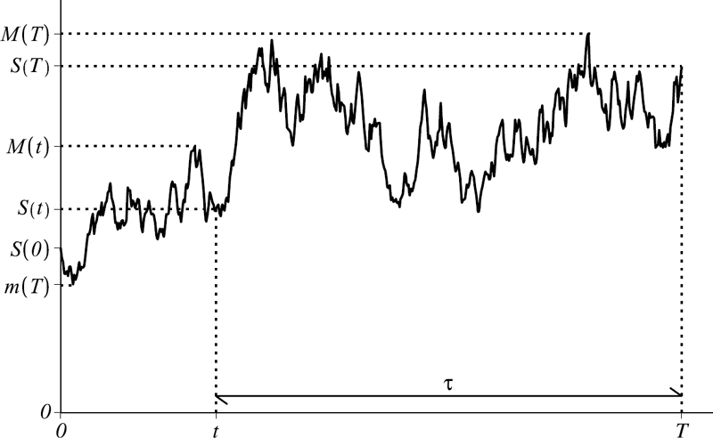
A sample stock price path is shown with its initial value, its value and realized maximum and minimum at both the intermediate (current) time t and at terminal time T.
Let’s now specialize to the case where the realized maximum and minimum are computed starting from current time t. Then S(t) = MS(t) = MS(t), i.e., with spot values S = M = m, where in the integrands of (12.111) and (12.112) we have, respectively,
Hence both payoff functions in (12.111) and (12.112) have the form φ(S eσw,S eσx) and the option pricing formulae are functions of only the spot S and τ = T − t. In particular, the pricing formula in (12.111) is reduced to V(t, S, M) = V(t, S) = ν(τ, S):
Setting the current calendar time t = 0, S = S(0) = S0, τ = T gives the price expressed as function of spot S0, and the time to maturity, which is now represented by the variable T, V(0, S0) = ν(T, S0):
Of course, we need only compute one of these as (12.114) obtains trivially from (12.113) and vice versa. For options involving the realized minimum, (12.112) gives V(t, S, m) = V(t, S) = ν(τ, S):
or expressed as a function of T and S(0) = S0, where we simply make the variable replacements S → S0 and τ → T in the derived pricing function ν(τ, S).
12.3.2 Pricing Single Barrier Options
For barrier options the contacts are specified such that the sampling of the maximum and minimum of the stock price starts at current time t. So we have the case discussed above where S(t) = MS(t) = mS(t) (or S0 = S(0) = MS(0) = mS (0) for current time t = 0). Hence the pricing formulae in (12.113)–(12.115) are our general starting point. Given a spot value S(t) = S, we denote the respective time-t pricing functions for cases (a)–(d) defined in (12.96) by VUO(t, S; B), VDO(t, S; B), VUI(t, S; B), and VDI(t, S; B). As functions of time to maturity we write these pricing functions equally as νUO(τ, S; B), νDO(τ, S; B), νUI(τ, S; B), and νDI(τ, S; B). By knock-in-knock-out symmetry in (12.98), we need only derive a pricing formula for either knock-out or knock-in options as we can use the pricing formula for the standard (vanilla) option to obtain one pricing formula from the other:
where V(t, S) is the time-t pricing formula for the standard European option with payoff function Λ.
For barrier options we see that the overall payoff function φ in all cases (a)–(d) in (12.96) is a product of an indicator function in the first argument and the effective payoff function Λ in the second argument. Hence, in the integrand of (12.113)–(12.115) we have in the respective cases (a)–(d) in (12.96):
where . These are all product functions in the integrand variables x and w. This leads to an important simplification in (12.113–(12.115) which reduce to single integrals, as given in the following result where the pricing formulae for knock-out barrier options are single integrals (in x) involving the effective payoff Λ(S eσx) and the risk-neutral probability density for the drifted BM in (12.101) that is killed at the effective barrier level b.
(Pricing Formulae for Single-Barrier Knock-Out Options). Assume a constant interest rate r and constant continuous dividend yield q on a stock whose price process is a GBM with constant volatility σ. Let B > 0 be an arbitrary knock-out barrier level, S(t) = S > 0 be the stock spot price, and Λ(·) be the effective payoff function. Then, for S < B the up-and-out option has value
and VUO(t, S; B) ≡ 0 for S ≥ B. For S > B, the down-and-out option has the value
and VDO(t, S; B) ≡ 0 for S ≤ B, where τ = T − t > 0 is the time to maturity, , , and is the (risk-neutral) density,
defined on the respective domains (−∞, b) and (b, ∞).
Proof. We prove (12.118), as (12.119) follows similarly. Using (a) in (12.117) within (12.113), changing the order of integration and evaluating the inner integral (as was done in (10.73) of Section 10.4.3 of Chapter 10):
for b > 0 and is identically zero for b ≤ 0, i.e., VUO(t, S; B) ≡ 0 for S ≥ B. Here we made use of (10.77) and (10.80) of Section 10.4.3 of Chapter 10, with the variable replacements for the drift µ → ν and level m → b. Note that
[Remark: The prices νUO(T, S0; B) = VUO(0, S0; B) and νDO(T, S0; B) = VDO(0, S0; B), expressing the current time-0 price with maturity T, follow in the obvious manner by setting t = 0, i.e., replacing τ → T and S → S0 in the above formulae.]
Note that the density function in (12.120) is a linear combination of two normal densities. Hence, to apply (12.118) or (12.119) we need to compute an integral of the function g(x) := Λ(S eσx), times ?{x<b} or ?{x>b}, against a normal PDF in x. Let’s now consider pricing an up-and-out call option where
and we assume the nontrivial case with S < B. Substituting this expression into the integrand in (12.118) gives the price of the up-and-out call as a difference of two integrals:
if , i.e., K < B. Note that CUO(t, S, K; B) ≡ 0 if κ ≥ b (i.e., K ≥ B). It is also clear from Figure 12.3 that paths which are in the money (above the strike) are necessarily above or at level B. Since all paths give zero payoff, the price of the up-and-out call must be identically zero when K ≥ B. For K < B the price is given by computing the two integrals in (12.122) upon substituting the density in (12.120). The second integral in (12.122) is a combination of two integrals involving the standard normal PDF which are readily evaluated by changing variables or simply using either identity (A.1) or (A.2) in the Appendix:
We can now express this in terms of the original parameters B, K, S, r, q, σ using (12.121) and the algebraic relations
where we define , . Substituting these expressions into (12.123) and using the identity gives the exact integral:
We leave it as an exercise for the reader to apply similar steps to show that the (discounted) first integral in (12.122) is given by
Substituting the integral expressions in (12.124) and (12.125) into (12.122) and combining terms gives the analytically exact pricing formula for the up-and-out call for K < B:
where
is the Black–Scholes pricing formula for a standard call on a dividend paying stock and CUI is the up-and-in call pricing formula for K < B:
where τ = T − t is time to maturity. Note that for K ≥ B, CUI(t, S, K; B) = C(t, S, K).
Pricing formulae for other up-and-out (and up-and-in) options are readily derived using similar steps and by combining the above integral identities in (12.124) and (12.125) within (12.118). For down-and-out (and down-and-in) we use (12.119) and develop similar identities to (12.124) and (12.125) for evaluating the pricing integrals. The derivations of pricing formulae for down-and-out (and down-and-in) call and put options are left as exercises at the end of this chapter.
(Up-and-Out Put Price) Derive the time-t, t < T, no-arbitrage pricing formula of an up-and-out put option with payoff
where B > 0 is the knock-out barrier and K > 0 the strike. Assume the stock is a GBM with constant interest rate and continuous dividend yield q.
Solution. We take spot S < B. For an up-and-out option we use (12.118) with put payoff
The integral over the density is restricted to . Since ?{x<κ}?{x<b} = ?{x<b∧κ},
where . The price of the up-and-out put is then given by
There are two cases: (i) B < K or (ii) B ≥ K. For B < K, b ∧ κ = b and the price is
The two integrals can be computed using the same steps and identities used for the up-andout call above. However, there is a shortcut based on (12.124) and (12.125) in the limit that the lower point of integration goes to −∞. That is, the above two integrals correspond to taking the limit , in the expressions in (12.124) and (12.125). Since , all terms with these arguments approach , as K → 0+. Upon using the symmetry in the resulting expressions we obtain:
and
Substituting these integrals gives the explicit pricing function for B < K:
τ = T − t. For B ≥ K, κ ≤ b, b ∧ κ = κ and the price is given by
In this case we express each integral on (−∞,κ) as the integral on (−∞, b) minus the integral on (κ, b). Then, we can use the difference of (12.128) and (12.124) to obtain the first integral on (−∞, κ) and the difference of (12.129) and (12.125). Combining terms and simplifying, we have the explicit pricing function for B ≥ K:
τ = T − t, where is the Black–Scholes pricing formula for a standard put on a dividend paying stock.
In closing this section we show that barrier options can also be “delta hedged” and we also make the connection between the risk-neutral pricing approach and the corresponding Black–Scholes PDE (BSPDE) for pricing single barrier options. We focus our discussion on the up-and-out and down-and-out options. The analysis for knock-in barrier options follows from knock-in-knock-out symmetry. As we have shown above, the general pricing formulae for the knock-out options are given by (12.118) and (12.119) of Proposition 12.1. Assuming that the integrals in (12.118) and (12.119) exist, and that we can evaluate them, we have completely solved the pricing problem for single barrier options. Alternatively, we now show that the pricing function is a solution to a BSPDE subject to appropriate boundary conditions. We have already seen how the risk-neutral pricing formulation is related to the BSPDE for the case of a standard (no barrier) European option. In particular, the pricing function V(t, S) in (12.15) is expressed as an (expectation) integral of the payoff against the risk-neutral transition PDF in (12.16) for the stock price process on the domain (0, ∞). The discounted risk-neutral transition PDF, and therefore V(t, S), solves the BSPDE (12.51) in the variables (S, τ) and (12.52) in the variables (t, S).
To see how the BSPDE arises for an up-and-out option, we apply a change of integration variables by letting in (12.118), which then takes the form
where is defined for all S, y values on the interval (0, B):
As shown in Exercise 12.22, this is the risk-neutral transition PDF for the stock price process killed at the first-hitting time to level B on either interval (0, B) or (B, ∞). The latter interval is used for the down-and-out option where (12.119) takes the same form as in (12.132) but with (B, ∞) as the integration interval in place of (0, B).
For any fixed y, the discounted transition PDF, , solves the time-homogeneous BSPDE in (12.51) subject to the initial condition ν(0+, S, y) = δ(S − y) (with the Dirac delta function δ). In fact, it is a fundamental solution on the interval (0, B) (as well as on the interval (B, ∞)) with zero boundary conditions at the barrier level B and at either endpoint S → 0+ or S →∞. Assuming the integral in (12.132) exists and the resulting pricing function is C1,2 (continuously differentiable in t (or τ) and twice differentiable in S), we can apply the differential operator (acting on variables t and S) on both sides of (12.132). Note that ℒBS is the Black–Scholes operator as in (12.52). By interchanging the order of differentiation and integration (in the dummy variable y), and using the fact that ν(τ, S, y) solves the BSPDE, gives
Hence, VUO ≡ VUO(t, S; B) is a solution to the BSPDE in (12.52) on the rectangular domain 0 < S < B, 0 ≤ t < T or equivalently the BSPDE in (12.51) for 0 < S < B, τ ∊ (0, T]. The terminal condition (or initial condition τ → 0+) is given by the payoff function where VUO(T, S; B) ≡ VUO(T −, S; B) = Λ(S), for any continuous Λ and for 0 ≤ S ≤ B. The boundary conditions at the endpoints of (0, B) are given by (note: S = 0 is the limit S ↘ 0)
The boundary condition at S = 0 is due to the stock price staying at zero if it is set to zero and hence the payoff will be Λ(0), which is discounted by e−r(T −t) to obtain its time-t value. The second condition corresponds to the option being worthless if the spot is at the barrier level any time before maturity. As an example, for an up-and-out call its value at the lower boundary S = 0 is CUO(t, 0, K; B) = e−r(T −t)Λ(0) = e−r(T −t)(0 − K)+ = 0 and at S = B we have CUO(t, B, K; B) = 0. For an up-and-out put, PUO(t, 0, K; B) = e−r(T −t)(K − 0)+ = e−r(T −t)K and PUO(t, B, K; B) = 0 at S = B.
For a down-and-out option the analysis is similar, leading to the same BSPDE in (12.52) for VDO ≡ VDO(t, S; B) on the rectangular domain B < S < ∞, 0 ≤ t < T or equivalently the BSPDE in (12.51) for B < S < ∞, τ ∊ (0, T]. The terminal (or initial) time condition is again the payoff function, VDO(T, S; B) = Λ(S), for B S < ∞, and with boundary endpoint conditions:
The first condition states that the value of the down-and-out option and the corresponding standard option value V(t, S) should be the same in the limit of infinite stock value. This is due to the stock price staying close to infinity and not hitting the lower knock-out barrier (in finite time) if it starts close to infinity. For the GBM model this is the case where the boundary at infinity is a natural boundary. The second boundary condition is again due to the option expiring worthless if the spot is at the barrier level before maturity. For example, a down-and-out call has value CDO(t, B, K; B) = 0 at S = B and . For a down-and-out put, PDO(t, B, K; B) = 0 and PDO(t, S, K; B) ~ P(t, S, K) ~ 0, as S → ∞.
Let V(t, S; B) denote either pricing function VUO(t, S; B) or VDO(t, S; B). For any given B > 0, we argued above that V(t, S; B) is a C1,2 function that solves the BSPDE in the (dummy) variables t, S. We can therefore apply Itô’s formula to the discounted process defined via the function V(t, S; B), i.e., {e−rtV(t, S(t); B)}t≥0. Taking the stochastic differential and using the fact that V(t, S; B) solves the BSPDE gives
Note that this stochastic differential and that of the discounted price process for the knockout barrier option are the same for all times before the stock price hits the barrier level B. Equating this with the expression in (12.7) gives the hedging position . For a given realization of the stock price process, this is then the hedging position held in the stock for all times t up to the first hitting time to the (knock-out) level B, or otherwise up to maturity time T if the stock price does not attain the level B during the option’s lifetime. In particular, for every spot value S(t) = S < B, the hedging formula for an up-and-out option is the delta of the pricing function, . Similarly, for S(t) = S > B, a down-and-out option is hedged using .
12.3.3 Pricing Lookback Options
We can now proceed to derive pricing formulae for generally “seasoned” lookback options of types (a)–(d) with payoffs defined in (12.99) where conditioning is on knowledge of the sampled stock price maximum, MS(t) = M ≥ S, or minimum mS(t) = m ≤ S, i.e., we are entering the contract at time t where the realized maximum or minimum up to time t generally differs from the stock (spot) price S(t) = S. Our main pricing formulae are (12.111) and (12.112). We therefore need the effective payoff functions in the integrand of either case. For example, consider the floating strike (LFS) call with payoff CTL F S = φ(mS (T), S(T)) = S(T) −mS(T) in (a) of (12.99), i.e. φ(x, y) := y − x. Hence, the effective payoff for this option is the integrand function in (12.112) given by
where . For case (b) in (12.99) we have φ(MS(T), S(T)) = MS(T) − S(T), i.e., φ(x, y) := x − y. Hence, the effective payoff in (12.111) is
where
The reader can verify that the effective payoffs for cases (c) and (d) are as given below where we summarize the effective payoffs for lookbacks (a)–(d) in (12.99):
where .
It is important to note that the functions in (c) and (d) depend only on w (not x). Moreover, the functions in (a) and (b) are simply sums of functions that depend on only one of the variables, either x or w and not both. This therefore simplifies the pricing integrals in (12.111) and (12.112), which are then sums of single integrals involving either (risk-neutral) marginal density in mX(τ) or MX(τ). Recall that integrating a joint PDF in one of its arguments (over ℝ) produces the corresponding marginal PDF. This simplification is given explicitly below for the above cases (a)–(d) where the pricing formulae are reduced to single integrals involving the marginal CDF or PDF of mX(τ) and MX(τ) and other more trivial integrals for the expected value of the drifted BM.
We now state these CDFs and PDFs for further use below when computing expectation integrals within the -measure. The CDFs of mX(τ) and MX(τ) were derived in Section 10.4.3 of Chapter 10. Under the risk-neutral measure we simply take the expressions in (10.82) and (10.88) where the process X now has drift and the time variable is τ, i.e., replace µ → ν, t → τ, and m → w in (10.82) and (10.88) to give
for w ≤ 0, and
for w ≥ 0. Differentiating these CDFs gives the densities, i.e., and , where
Alternatively, the reader can verify that these same expressions are obtained by successively integrating the respective joint PDFs in (12.108) and (12.109).
Based on (12.111) and (12.112), we can now derive the main pricing formulae for the above four types of lookback options. Consider case (a), where we denote the time-t pricing function for the LFS call by CL F S(t, S, m) for all 0 < m ≤ S < ∞. Substituting (12.137) into (12.112) gives this pricing function as a sum of three integrals involving the joint PDF . The integrals are respectively reduced to single integrals involving the marginal PDF of X(τ) and of mX(τ) as follows:
The integrals are recognized as expectations, where the third integral is :
The first expectation is computed simply as . This holds true even for more complex models as long as the stock price S(t) discounted by e−(r − q)t is a -martingale. Hence, the pricing formula for the LFS call is given equivalently by:
where τ = T − t. In the second equation line we have the respective quantities expressed in terms of mS(τ), and since the sampled minimum of the stock price (started at spot value S) for a time interval τ is . The third line is obtained by re-expressing the expectation in the second line upon using an integration by parts,
This identity is valid for any number m 0.
A similar derivation follows for the floating strike lookback (LFS) put option defined by the payoff in case (b) above where we denote the time-t pricing function for the LFS put by PL F S(t, S, M), for all 0 < S ≤ M < ∞. We now substitute (12.138) into (12.111) and this leads to a sum of three integrals involving the joint PDF of . Using similar steps as above, the reader can verify that the resulting pricing formula takes the equivalent expressions:
τ = T − t. In the second equation line we have the respective quantities expressed in terms of and since the sampled maximum of the stock price is . The third line is obtained by noting that , where . The expected value of the positive random variable MS(τ) can be represented as an integral over its right tail (risk-neutral) probability:
The expected value of can be expressed by applying an integration by parts procedure as above,
Since , for any y ≥ 0, we can write the last integral as , and then combine the above two expectations to establish the identity
for any number M ≥ 0. Substituting this into the second line of (12.148) gives the expression in the third line of (12.148). For the payoff in case (c) above we denote the time-t pricing function for the floating price lookback (LFP) call (on the maximum) with strike K > 0 by CL F P(t, S, M; K), for all 0 < S M < ∞. By using similar steps as in case (b) above, the reader can verify that the pricing formula takes on the equivalent expressions:
for M ≥ K, and
for M < K, where τ = T − t. Note that for M < K the pricing function CL F P , given by (12.150), is independent of the realized maximum M of the stock price at current time t.
In the last case (d) we denote the time-t pricing function for the floating price lookback (LFP) put (on the minimum) with strike K > 0 by PL F P(t, S, m; K), for all 0 < m ≤ S < ∞. By using similar steps as in case (a) above, the reader can verify that the pricing formula takes the equivalent forms:
for m ≥ K, and
for m < K, where τ = T − t. Note that for m ≥ K the pricing function PL F P in (12.151) is independent of the realized minimum m of the stock price at current time t.
The relations in (12.147)–(12.152) can therefore be used to price all four main types of lookback options. These relations are valid for quite general (time-homogeneous Markov) models for the stock price with discounted process {e−(r − q)tS(t)}t≥0 assumed to be a -martingale. Of course, within the GBM model we have simple exact explicit formulae for all the necessary PDFs and CDFs that can now be used to derive analytically exact risk-neutral pricing formulae for all four types of lookback options. For instance, Example 12.5 below gives a derivation of PL F S(t, S, M) by implementing (12.148) within the GBM model for the stock price. Before presenting this example, we note that the pricing relations in (12.147), (12.148), (12.149), and (12.152) also further simplify in the case where the sampling of the maximum and minimum is started at the current time t: S(t) = MS(t) = mS(t). This is seen by setting M = S and m = S and noting that mS(τ) < S and MS(τ) > S (a.s.), i.e., the probability becomes and becomes . Moreover, the indicator functions simplify where becomes and becomes . This is consistent with the fact that and when M = m = S. All the pricing formulae are then only functions of spot S and time t (or S and τ).
(Floating Strike (LFS) Put Price) Derive the no-arbitrage pricing formula PL F S(t, S, M) for the lookback option with payoff (b) in (12.99). Assume the stock price is a GBM with a constant interest rate and a continuous dividend yield q.
Solution. It is convenient to obtain the pricing function PL F S(t, S, M) by using the first equation line in (12.148). The first term is evaluated explicitly by evaluating the CDF in (12.141) at and using the drift parameter ,
where we define ; x > 0, τ = T − t > 0. Note that .
We now need to compute the (expectation) integral in (12.148). By substituting the density in (12.143), the integral is a sum of three integrals:
The first two Gaussian integrals are readily evaluated by completing the square in the exponents, or simply by direct use of the integral identity (A.1) of the Appendix. It turns out that both integrals are given by
Note that . So the third integral can be evaluated in two separate cases: (i) r − q = 0 and (ii) r − q ≠ 0. We will treat the latter case since the pricing formula for case (i) can be obtained by taking the limit (r − q) → 0 in the pricing formula for case (ii).
We now evaluate the third integral using a change of variables, , and write , giving
Note that . Here we define the constants and . We can assume that r − q > 0, i.e., A < 0, so that the integral identity in (A.5) of the Appendix can be directly applied. [We leave it to the reader to apply a change of variable and verify that the same result obtains by making use of an appropriate integral identity in the Appendix for the case that r − q < 0.] Applying (A.5) and simplifying the terms gives
Substituting this expression into (12.156) and summing the resulting expression with the two equal expressions in (12.155) gives the left-hand side integral in (12.154):
Finally, by inserting this expression and the CDF in (12.153) into (12.148) and cancelling out two terms gives the pricing function for r − q ≠ 0:
The pricing formula for r − q = 0, i.e., when r = q, follows by taking the limit r − q → 0. We leave it as a simple exercise in calculus (using L’Hôpital’s Rule) to show that the sum of the two terms in cancel out when r − q → 0. Then, using r = q, the final expression for the pricing function in case r − q = 0 simplifies to
where .
In the above example, if we assume that the sampling of the maximum starts at current time t, i.e., S = M, then the pricing formulae in (12.158) and (12.159) simplify to
for r ≠ q and
for r = q, where we simply write PL F S(t, S) ≡ PL F S(t, S, M = S). The pricing functions in (12.160) and (12.161) are simply linear functions in S.
The derivations of explicit pricing functions for the other lookback options are left as exercises at the end of this chapter (see Exercise 12.24).
12.4 Exercises
Exercise 12.1. Let the stock price process {S(t)}t≥0 be a geometric Brownian motion (GBM) with constant volatility σ. Assume a constant continuous dividend yield q on the stock and a bank account with constant continuously compounded interest rate r. Fix S(0) = S > 0 and time T > 0. Let the process {e(q−r)tS(t)}t≥0 be a -martingale. Derive explicit analytical expressions for the risk-neutral probability of the following events:
- (a) {S(T) < K}, with constant K > 0;
- (b) {K1 < S(T) < K2}, with constants K2 > K1 > 0;
- (c) {1/S2(T) > K}, with constant K > 0;
- (d) {Sα(T2) > Sβ(T1)}, with times T2 > T1 > 0 and constants α, β ≠ 0;
- (e) {S(T2) > S(T1) > S(t)}, with times T2 > T1 > t > 0;
- (f) {S(T1) < K1, S(T2) > K2} for any K1, K2 > 0.
Exercise 12.2. Assume the standard Black–Scholes model in an economy with constant continuously compounded interest rate r and with stock price process {S(t)}t≥0 as a GBM with constant volatility σ and constant continuous dividend yield q. Derive the no-arbitrage pricing formula for the European-style option with the corresponding payoff functions (a)– (c), where K > 0 is a fixed strike and a > 0 is a constant. Express your answer in terms of the spot S and the time to maturity.
- (a) Λ(S) = a(S − K)2;
- (b) Λ(S) = (aS2 − K)+;
- (c) Λ(S) = a|Sα − K| with nonzero real constant α.
Exercise 12.3. Assume the standard Black–Scholes model and stock price process as in Exercise 12.2. Consider a European option with payoff at expiry T:
where K1 < X1 < X2 < K2 and X2 = K1 + K2 − X1.
- (a) Give a sketch of this payoff function and determine a replicating portfolio for Λ(S(T)) that consists of only calls or puts.
- (b) Let S(t) = S be the spot price of the stock at current time t < T. Derive the risk-neutral pricing formula for the time-t value of a European-style option with the above payoff function. Give an explicit answer in terms of all parameters in the model.
- (c) Obtain a formula for the delta position in the stock at time t < T that is required in a self-financing replicating strategy for the option.
Exercise 12.4. Assume the standard Black–Scholes model and stock price process as in Exercise 12.2. Let S(t) = S > 0 be the spot at time t < T, where T is the expiry date. Derive the corresponding arbitrage-free time-t pricing formula, V(t, S), for a European option with the respective payoffs in (a) and (b) below.
- (a) , where an are real constant coefficients of the polynomial function.
- (b) Λ(S(T)) = Sα(T) − K ?{S(T)>K} where α is any nonzero real constant.
Exercise 12.5. Assume the standard Black–Scholes model and stock price process as in Exercise 12.2. A European call spread has payoff Λ(S(T)) equal to zero for S(T) ≤ K, S(T) − K for K < S(T) < K + ∊, and ∊ for S(T) ≥ K + ∊, where K, ∊ are any positive values.
- (a) Give a sketch of the payoff function.
- (b) Derive a formula for the option’s present value V(t, S) and . Express your answers in terms of spot S, time to maturity T − t, and parameters K,∊,r,q,σ.
- (c) Find V(t, S) in both limits ∊ ↘ 0 and ∊ → ∞ and explain your results.
Exercise 12.6. Let 0 < K1 < K2 < K3 < K4 < K5 < K6 and consider the payoff function:
where we assume K4 − K3 > K2 − K1 and K2 − K1 − (K4 − K3) = K5 − K6.
- (a) Give a sketch of this payoff function.
- (b) Determine a replicating portfolio for Λ(S) consisting of only calls (or puts, cash, and stock positions).
- (c) Assuming a Black–Scholes economy as in Exercise 12.2, derive the no-arbitrage pricing formula for the European-style option with the above payoff.
Exercise 12.7. A so-called range forward European contract is specified as follows: at maturity T the holder must buy the underlying stock at price K1 if S(T) < K1, at price S(T) if K1 ≤ S(T) ≤ K2, and at price K2 for S(T) > K2 where K1 < K2 are fixed strikes.
- (a) Derive the explicit formula for the present value V(t, S) of this contract with spot S(t) = S. Assume a Black–Scholes economy as in Exercise 12.2.
- (b) Find the relationship between K1 and K2 such that the present value V(t, S) = 0.
Exercise 12.8. Consider a so-called strangle payoff function Λ(S) defined by two strikes 0 < K1 < K2:
- (a) Give a sketch of Λ(S).
- (b) Determine a replicating portfolio for Λ(S) in terms of positions in standard calls, stock, and cash.
- (c) Assume the stock price {S(t)}t≥0 is a GBM with constant volatility σ, constant continuous dividend q in an economy with constant interest rate r. Derive the arbitrage-free pricing formula for the present time t < T value of a European-style derivative with the above payoff function.
- (d) Provide an expression for the value, at calendar time t < T, of the position in the stock in the self-financed portfolio required to dynamically replicate the option value.
- Exercise 12.9. A so-called pay-later European option costs the holder nothing (i.e., zero premium) to set up at present time t = 0. The payoff to the holder at maturity T > 0 is (S(T) − K)+. Moreover, the holder must pay out X dollars to the writer in the case that S(T) ≥ K. Derive an expression for the fair value of X. Determine the fair value for X in the limit of infinite volatility, σ → ∞. Assume a Black–Scholes economy as in Exercise 12.2.
Exercise 12.10. Let C(S, τ) be the Black–Scholes pricing formula of a standard call option with spot S, strike K, fixed interest rate r, zero stock dividend, constant volatility σ, and time to maturity τ > 0.
(a) Show that the respective limiting values of the call price for vanishing and infinite volatility are given by
- (b) Give a financial interpretation of both limits. Note that the second limit is independent of the strike value K; give a financial intuition of this fact.
Exercise 12.11. Consider the value of a European call option written by an issuer who only has a fraction 0 ≤ α < 1 of the underlying asset. That is, at expiration time T the payoff of this type of call is given by
Let CL(S, τ; K, α) denote the value of such a European call, where τ = T − t is the time to expiry, K > 0 is the strike, S(t) = S is the spot of the underlying. Show that
where is the price of a standard European call with strike , spot S, and time to expiry τ. NOTE: You should not assume any model for the stock price process and therefore you need not provide any explicit formulas for any of the call price functions.
Exercise 12.12. Suppose that the cost of carry on a commodity is b and assume a bank account with constant interest rate r. Let the price of the commodity follow a GBM model with constant volatility σ. Let V = V(t, S) be the value of a European option on this commodity, where S > 0 is the spot value of the commodity at calendar time t.
(a) Show that V satisfies the Black–Scholes PDE:
- (b) Based on (a), find the put-call parity relation between the put price P(t, S) and call price C(t, S), with common strike K and time to maturity τ = T − t.
Exercise 12.13. Consider a portfolio Π with fixed positions θi in N securities each with price fi, i = 1, ..., N, respectively. Assume the ith security has price fi as a function of the same spot S at current time t and that each fi = fi(S, Ti − t) satisfies the time-homogeneous Black–Scholes PDE with constant interest rate and volatility. The contract maturity dates Ti are allowed to be distinct. Find the algebraic relationship among the portfolio Greeks: .
Exercise 12.14. Apply integration by parts twice to show that
is an integral representation of the payoff in (12.43). Hence, this shows that the soft-strike call option with given central strike K and strike width a > 0 is replicated as a uniform superposition of standard call options of all strikes in the interval (K − a, K + a).
Exercise 12.15. Recall the pricing of the soft-strike call in Example 12.2.
- (a) Provide the corresponding definition of the payoff (as in (12.43)) of the soft-strike put option with center strike K and width a. Provide a plot of the payoff and describe its main features as done in Example 12.2.
- (b) Derive a corresponding put-call parity relation for the soft-strike call and soft-strike put options having common center strike K and strike width a. Assuming the standard GBM model as in Example 12.2, derive the formula for P(t, S; K, a), the no-arbitrage time-t price of the soft-strike put option.
Exercise 12.16. Assume the risk-neutral pricing formula in (12.11) holds. By using a general formula for the expectation of a random variable conditional on an event, in this case the event {S(T) > K}, derive the following general representations for the respective prices of a standard call and put option with strike K:
Exercise 12.17. Assume a nondividend paying stock with price process {S(t)}t≥0 as a GBM with constant volatility σ > 0 in the (B, S) economy with constant interest rate r. Let Ct := C(t, S(t), K) be the price process at calendar time t, 0 ≤ t < T, with C(t, S, K) as the pricing function of a standard European call option on the stock with given strike K > 0 and fixed maturity date T. It follows that Ct satisfies the SDE
where is a standard BM under the risk-neutral measure .
(a) Find explicit expressions for µc and σc, i.e., the (log)-drift and (log)-volatility coefficient functions of the call price process.
NOTE: The (log)-volatility of the call price, σc, is a function of S(t) (spot value) and parameters K, σ, r, τ = T − t. Your expressions should be simplified as much as possible. Define all terms in your answer.
- (b) Find the limiting expression for σc as K ↘ 0 (holding spot and other parameters fixed). Give a financial explanation of the resulting limit.
Exercise 12.18. Consider a stock price process as a GBM and assume deterministic (nonrandom) time-dependent volatility σ(t), stock dividend yield q(t), and interest rate r(t). Assume that these are integrable functions of time t ∊ [0, T].
- (a) Derive the time-0 no-arbitrage pricing function C(0, S0, K) for the standard call option on this stock with S(0) = S0 > 0 as spot, K > 0 as strike, and T as maturity.
- (b) Derive the put-call parity relation between the time-0 values of the standard call and put prices C(0, S0, K) and P (0, S0, K).
- (c) Now let the present time be any time t ∊ [0, T) with spot S(t) = S > 0. Derive the time-t no-arbitrage pricing function for the standard call C(t, S, K) and provide the corresponding put-call parity relation where P(t, S, K) denotes the time-t pricing function for the standard put.
Exercise 12.19. A variant of the forward starting call option that we already considered in Section 12.2 is structured as follows. The holder receives at date T1 > t a call with strike and maturity T > T1. Here, α is a positive constant and S(T1) is the stock price realized at time T1. Let the stock price be a GBM with constant interest rate r and dividend yield q.
- (a) Let S(t) = S. Derive the time-t pricing formula C(t, S; T1, T) for this forward starting call and give a hedging strategy that applies up to time T1. Is the strategy static or not?
- (b) Show that the price of the forward starting call simplifies to that of a standard call struck at K = αS with time to maturity T − t in the limiting case that T1 → t (with t, T held fixed). On the other hand, show that in the limit T → T1 (with t, T1 held fixed) the contract price is simply given by S(1 − α)+.
Exercise 12.20. Assume the stock price {S(t)}t≥0 is a GBM with constant volatility σ and zero dividend in an economy with constant interest rate r. Let t < T0 < T , i.e., T0 is an arbitrary intermediate time before expiry time T, and consider a European-style option with payoff at time T:
(a) Show that the value V at any time t ≤ T0 of this option is given by
where S(t) = S is the spot and .
[Note: The option value is dependent on T − T0 (where T and T0 are fixed) and does not depend on t.]
- (b) What is the position held in the stock at time t ≤ T0 in a self-financing replicating strategy? Is this position static over time? Justify whether or not a bank account is needed in the dynamic replication.
Exercise 12.21. Recall the derivation of the pricing function Vcc(t, S) for the European call-on-a-call where S(t) = S is the spot at calendar time t < T1 < T2. Assume the stock price is a GBM with constant interest rate r and constant dividend yield q.
- (a) Using similar steps as in Section 12.2, derive the pricing formula for Vcp(t, S), the arbitrage-free value of a call-on-a-put, with time-T1 value , where is the price of the (embedded) standard put with time to maturity T2 − T1 and strike K2.
- (b) Derive an expression for the delta position Δt = Δ(t, S) in the stock at time t < T1 needed to dynamically hedge the call-on-a-put option in (a).
Exercise 12.22. Consider the stock price process {S(B)(t)}t≥0 as a GBM that is killed at the first-hitting time TBS = inf{t ≥ 0: S(t) = B} to level B > 0:
where S(t) is given by (12.100) and X(t) is given by (12.101). Note that the state space for the process is restricted to either interval (0, B) or (B, ∞) corresponding to the two cases with S(0) ∊ (0, B) or S(0) ∊ (B, ∞), respectively.
(a) Show that the transition CDF for the process S(B) is given by
where τ = T − t > 0 and X(b) is the BM process given by (12.101) with killing at the first-hitting time to level (see the definition in (10.75) of Chapter 10). By differentiating, obtain the (time-homogeneous) transition PDF:
where and is the risk-neutral transition PDF for the killed BM process X(b). Then, using the density in (12.120), obtain the expression in (12.133).
- (b) For a fixed y value, show that solves the time-homogeneous BSPDE in (12.51) subject to the initial condition ν(0+, S, y) = δ(S − y) and has zero boundary conditions ν(τ, S = B, y) = 0 and ν(τ, S = 0+, y) = 0 and ν(τ, S = ∞, y) = 0 for all τ > 0 and all y.
Exercise 12.23. Using similar steps as in the derivation of the up-and-out call (and up-and-out put) pricing formula, derive explicit pricing functions and delta hedging positions for
- (a) the down-and-out put and down-and-in put option;
- (b) the down-and-out call and down-and-in call option.
Assume a barrier level B > 0, strike K > 0, time to maturity τ = T − t > 0 and where the stock price is a GBM with constant interest rate r and stock dividend yield q.
Exercise 12.24. Use similar steps as in Example 12.5 and make appropriate use of integral identities in the Appendix to derive explicit pricing functions for
Assume the stock price is a GBM with constant interest rate r and dividend yield q.
Exercise 12.25. Consider the discrete geometric averaging of a stock price process at evenly distributed discrete times tj = t0 + j δt, j = 1, 2, ..., n, with a time step δt = (T − t0)/n; tn = T is the time of expiration. Define the discretely monitored geometric averaging by
- (a) Assuming that the stock price follows a GBM process, show that Gn is a log-normal random variable. Find the mean and variance of Gn.
- (b) Derive the risk-neutral time-t0 prices of the fixed strike Asian call and put options with respective payoff functions (Gn − K)+ and (K − Gn)+. Here, K > 0 is a strike price.
Exercise 12.26. Let the stock price process follow the GBM model in (12.46). Define the continuously monitored geometric average of S(t) over a time period [0, t] by
- (a) Show that the process {ln G(t)}t≥0 is Gaussian.
- (b) Find the mean and variance of G(T) conditional on G(t) and S(t) for 0 ≤ t ≤ T.
(c) Show that G(T) can be written as
for some , and where under measure . Find the values of and .
- (d) Derive the risk-neutral time-t pricing functions for the fixed strike Asian call and put options with respective payoff functions (G(T) − K)+ and (K − G(T))+ for 0 ≤ t ≤ T. Express the pricing functions in terms of the spot values G(t) = G > 0, S(t) = S > 0, and times t and T.
- (e) Establish the put-call parity relation for the fixed strike Asian call and put options.
1 Assuming there is no confusion, when discussing pricing formulas we prefer to choose more appropriate letters for some of the ordinary variables. In this case we denote the spot value by using the dummy variable S, instead of using some other letter like x, in the context of a pricing formula.
2 It is also trivial to see in this case that the natural filtration generated by W (ℙ-measure BM) is the same as the natural filtration generated by W (-measure BM) since the two Brownian motions differ only by a constant: , so for every t ≥ 0.
3 In applying the expectation identities in the Appendix we need to simply identify the parameters A, B and the mean µ and variance σ2 of the appropriate normal random variable X in the given measure. Note that the parameter σ used in the above equations is obviously the symbol for the volatility of the stock. Of course, this σ is not the same σ used throughout the Appendix! For the expectation in (12.25), we employ the formula in (A.1) by identifying as and .
4 We remind the reader of the shorthand notation we have been adopting for conditional expectations. In particular, is a number where S > 0 is a spot value and is a σ(S(T1))-measurable (and hence -measurable) random variable where we are conditioning on the σ-algebra, σ(S(T1)), generated by the stock at time T1.