Table 17.3 Sample values for Figure 17.6
Cal Id | Mo Code | Mo Desc | Qtr Code | Qtr Desc | Yr Cd | Yr Desc | Level Cd |
1 |
|
|
|
| 2007 | Two Thousand Seven | Year |
2 |
|
|
|
| 2008 | Two Thousand Eight | Year |
3 |
|
|
|
| 2009 | Two Thousand Nine | Year |
4 |
|
| Q12009 | First Quarter Two Thousand Nine | 2009 | Two Thousand Nine | Quarter |
5 |
|
| Q22009 | Second Quarter Two Thousand Nine | 2009 | Two Thousand Nine | Quarter |
6 |
|
| Q32009 | Third Quarter Two Thousand Nine | 2009 | Two Thousand Nine | Quarter |
7 | Jan2009 | January Two Thousand Nine | Q12009 | First Quarter Two Thousand Nine | 2009 | Two Thousand Nine | Month |
8 | Feb2009 | February Two Thousand Nine | Q12009 | First Quarter Two Thousand Nine | 2009 | Two Thousand Nine | Month |
9 | Mar2009 | March Two Thousand Nine | Q12009 | First Quarter Two Thousand Nine | 2009 | Two Thousand Nine | Month |
Figure 17.7 Sales reporting with the Calendar FUBES structure

In Figure 17.7 we are summing and loading sales data at the month, quarter, and year levels. If there is a need to retrieve Annual sales for 2011, we can quickly find this number because we are storing the Sales Value Amount for 2011 in Annual Sales, which references the Calendar instance where Calendar Level Code equals ‘Year’ and Year Code equals ‘2011’.
 To apply FUBES, use the ‘Column Denormalization’ feature. Alternatively, replicate columns with the standard replication feature, although this will not appear in the list of model transformations.
Repeating Groups
In the repeating-groups technique, the same data element or group of data elements is repeated two or more times in the same entity. Also known as an array, a repeating group requires making the number of times something can occur static. Recall that in 1NF we removed repeating groups. Well, here it is, being reintroduced again. An example of a repeating group appears in Figure 17.8.
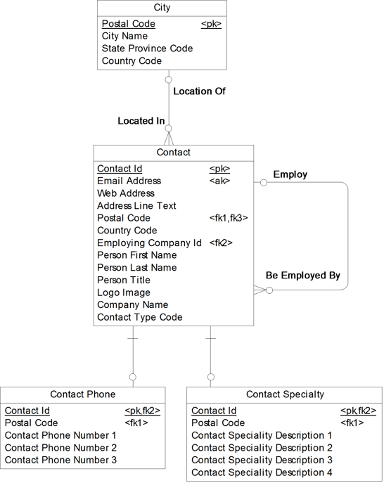
Figure 17.8 Repeating groups in our Contact example

In this example, we can have up to three phone numbers for a Contact and up to four specialties. In addition to choosing denormalization because of the need for faster retrieval time or for more user friendly structures, repeating groups may be chosen in the following situations:
· When it makes more sense to keep the parent entity instead of the child entity. When the parent entity is going to be used more frequently than the child entity, or if there are rules and data elements to preserve in the parent entity format, it makes more sense to keep the parent entity. For example, in Figure 17.8, if Contact is going to be accessed frequently, and when Contact is accessed, Phone Number and Specialty Description are also occasionally accessed.
· When an entity instance will never exceed the fixed number of data elements added. In Figure 17.8, we are only allowing up to three phone numbers for a contact, for example. If we have four phone numbers for Bob the Contact, how would we handle this? Right now, we would have to pick which three of them to store.
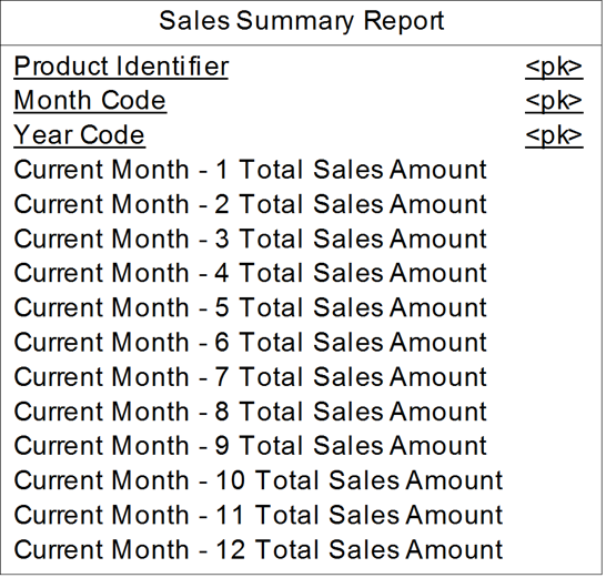
· When you need a spreadsheet. A common use is to represent a report that needs to be displayed in a spreadsheet format. For example, if a user is expecting to see a sales report in which sales is reported by month for the last 12 months, an example of a repeating group containing this information is shown in Figure 17.9. At the end of a given month, the oldest value is removed and a new value is added. This is called a rolling 12 months. Faster performance and a more user-friendly structure lead us to add repeating groups in this example and purposely violate 1NF.
Figure 17.9 Sales-report entity with repeating group
To apply the repeating groups technique, replicate columns with the standard replication feature – this will not appear in the list of model transformations.
Repeating Data Elements
Repeating data elements is a technique in which you copy one or more data elements from one entity into one or more other entities. It is done primarily for performance because by repeating data elements across entities, we can reduce the amount of time it takes to return results. If we copy Customer Last Name from the Customer entity to the Order entity, for example, we avoid navigating back to Customer whenever just Customer Last Name is needed for display with order information.
Repeating data elements differs from repeating groups because the repeating groups technique replaces one or more entities and relationships, while the repeating data elements technique retains the existing entities and relationships and just copies over the data elements that are needed. For example, to apply the repeating groups technique to Customer and Order, we’d need to determine the maximum number of orders a customer can place, then remove the Order entity and its relationship to Customer and repeat three or four or however many times all of the order data elements within Customer. The repeating data elements technique would just involve copying over the data elements we need and keeping everything else intact.
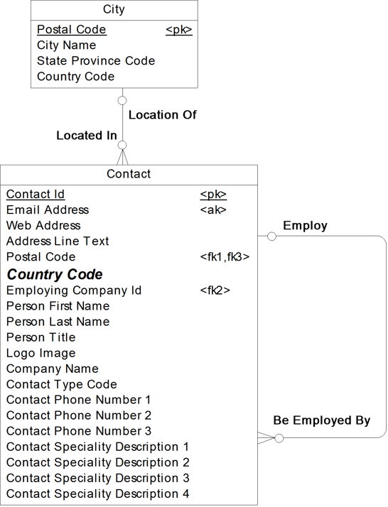
See Figure 17.10 for an example of this technique using our Contact example. In this example, there was a need to view the country along with contact information. Therefore, only the Country Code data element needed to be copied to Contact, while the City entity and its relationship remains intact.
 In PowerDesigner, you should use the ‘Column Denormalization’ feature to copy columns to child tables. The new column is a managed, read-only copy of the original – any changes made to the original column are automatically made to the denormalized copy of it. In fact, you cannot alter the copy column.
In addition to choosing denormalization because of the need for faster retrieval time or for more user friendly structures, repeating data elements can be chosen in the following situations:
· When the repeated data element or elements are accessed often and experience few or no changes over time. If, for example, Country Code changed frequently, we would be required to update this value on City and for each of the contacts related to City. This takes time to update and could introduce data quality issues if not all updates were performed correctly, completely, or on a timely basis.
· When the standard denormalization option is preferred, but space is an issue. There might be too huge an impact on storage space if the entire parent entity was folded up into the child and repeated for each child value. Therefore, only repeat those parent data elements that will be used frequently with the child.
· When there is a need to enforce the business rules from the LDM. With the repeating data elements technique, the relationships still remain intact. Therefore, the business rules from the logical data model can be enforced on the physical data model. In Figure 17.10 for example, we can still enforce that a Contact live in a valid City.
Figure 17.10 Repeating data elements in our Contact example
To apply the repeating data elements technique, use the column denormalization feature.
Summarization
Summarization is when tables are created with less detail than what is available in the business. Monthly Sales, Quarterly Sales, and Annual Sales from Figure 17.7 are all summary tables derived from the actual order transactions.
In addition to choosing denormalization because of the need for faster retrieval time or for more user friendly structures, summarization can be chosen when there is a need to report on higher levels of granularity than what is captured on the logical data model. Annual Sales for example, provides high level summary data for the user, and therefore the user (or reporting tool) does not have to spend time figuring out how to produce annual sales from detailed tables. The response time is much quicker because time does not need to be spent summarizing data when it is requested by a user; it is already at the needed summarization level, ready to be queried.
To apply the summarization technique, create a new summary table. To create similar tables, either copy or replicate the original. In Figure 17.7, for example, the Quarterly Sales and Annual Sales could be replicas of Monthly Sales. Any changes made to Monthly Sales (e.g. new columns) would also be made to the replicas. If you need the tables to have more independence, you can break the replication link at any time.
Star Schema
Denormalization is a term that is applied exclusively to relational physical models, because you can’t denormalize something unless it has already been normalized. However, denormalization techniques can be applied to dimensional models, as well - you just can’t use the term ‘denormalization’. So all of the techniques from the standard method through summarization can be used in dimensional modeling, just use a term such as ‘flattening’, instead of ‘denormalization’.
A star schema is the most common dimensional physical data model structure. The term ‘meter’ from the dimensional logical data model, is replaced with the term ‘fact table’ on the dimensional physical data model. A star schema results when each set of tables that make up a dimension is flattened into a single table. The fact table is in the center of the model, and each of the dimensions relate to the fact table at the lowest level of detail. A star schema is relatively easy to create and implement, and visually appears elegant and simplistic to both IT and the business.
Recall the dimensional logical modeling example from the previous chapter, copied here as Figure 17.11.
Figure 17.11 Dimensional logical data model of ice cream

A star schema of this model would involve folding Year into Month and Month into Date, and then renaming Date with a concept inclusive of Month and Year, such as ‘Time’ or ‘Calendar’. See Figure 17.12 for the star schema for this example.
Figure 17.12 Ice cream star schema

To create a star schema, use a combination of new tables and columns, and the FUBES and repeating data element techniques described above.
In Figure 17.12, I populated the Dimensional Type property on the ‘General’ tab for each Table. PowerDesigner automatically displays the icons in the top left corner of the table symbols. These tell you that Ice Cream Sales is a ‘Fact’ table, and that the other two tables are ‘Dimensions’. PowerDesigner also allows you to create special ‘Multidimensional’ diagrams, where Facts and Dimensions are objects in their own right, not just specialized tables. 
![]() “Building Multidimensional Diagrams”
“Building Multidimensional Diagrams”
Views Explained
A view is a virtual table. It is a dynamic “view” or window into one or more tables (or other views) where the actual data is stored. A view is defined by a query that specifies how to collate data from its underlying tables to form an object that looks and acts like a table, but doesn’t physically contain data. A query is a request that a user (or reporting tool) makes of the database, such as “Bring me back all Customer Ids where the Customer is 90 days or more behind in their bill payments.” The difference between a query and a view, however, is that the instructions in a view are already prepared for the user (or reporting tool) and stored in the database as the definition of the view, whereas a query is not stored in the database and may need to be written each time a question is asked.
Returning to our Contact example, let’s assume that the users continuously ask the question, “Who are the people that live in New Jersey?” We can answer this question in a view. Figure 17.13 contains the model from Figure 17.10 with the addition of a view to answer this question.
In many tools, a view is shown as a dotted box; PowerDesigner uses solid lines and rounded corners, instead. In this model, it is called Person In New Jersey. This view needs to bring together information from the entity City and from the entity Contact to answer the business question.
Figure 17.13 View added to answer business question
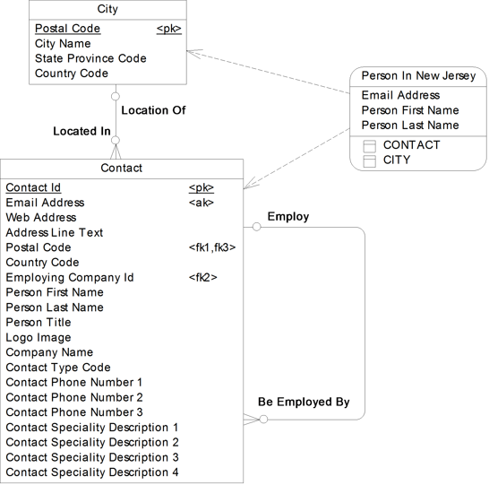
PowerDesigner records the interdependencies between the view and the tables, but doesn’t automatically create lines to illustrate those dependencies. In Figure 17.13, the dashed lines connecting the view to the table were added manually, as ‘traceability links’. This feature allows you to visually document any dependencies that matter to you.
The instructions to answer this business question are written in a query language a database can understand, usually in the language SQL (pronounced ‘sequel’). SQL is powerful for the same reason that data modeling is powerful: with a handful of symbols, one can communicate a lot. In English, the SQL statement in Figure 17.14 is saying “Give me the last name, first name, and email address of the Contact(s) whose postal code matches a postal code in the City table that has a state code of ‘NJ’, where the Contact is a person (and not a company)”.
Figure 17.14 SQL language to answer question “Who are my Contacts that live in New Jersey?”
select
CONTACT.EMAIL_ADDRESS,
CONTACT.PERSON_FIRST_NAME,
CONTACT.PERSON_LAST_NAME
from
CONTACT,
CITY
WHERE (CITY.POSTAL_CODE=CONTACT.POSTAL_CODE)
AND (CITY.STATE_PROVINCE_CODE=‘NJ’)
AND (CONTACT.CONTACT_TYPE_CODE = ‘PRSN’);
PowerDesigner allows you to define and preview the SQL for the query in the property sheet for the View, in the ‘SQL Query’ tab. It is also visible in the ‘Preview’ tab. PowerDesigner creates dependencies between the view and the objects that it accesses, based upon the SQL statements.
There are different types of views. Typically, execution of the view (i.e. the SQL statement) to retrieve data takes place only when a data element in the view is requested. It can take quite a bit of time to retrieve data, depending on the complexity of the request and the data volume. However, other types of views can match and sometimes even beat retrieval speed from actual tables, because their instructions are run at a predetermined time, with the results stored in the database, similar to a database table.
Views are a popular choice for assisting with security and user-friendliness. If there are sensitive data elements within a database table that only certain people in the company should have access to, then views are a great way to hide these sensitive data elements from the common user. Views can also take some of the complexities out of joining tables for the user or reporting tool.
In fact, we can use views in almost all situations where we are using denormalization. At times, views can offer all of the benefits of denormalization without the drawbacks associated with data redundancy and loss of referential integrity. A view can provide user-friendly structures over a normalized structure, thereby preserving flexibility and referential integrity. A view will keep the underlying normalized model intact, and at the same time present a denormalized or flattened view of the world to the business.
Indexing Explained
An index is a pointer to something that needs to be retrieved. An analogy often used is the card catalog, which in the library, points you to the book you want. The card catalog will point you to the place where the actual book is on the shelf, a process that is much quicker than looking through each book in the library until you find the one you need. Indexing works the same way with data. The index points directly to the place on the disk where the data is stored, thus reducing retrieval time. Indexes work best on data elements whose values are requested frequently, but are rarely updated.
Primary keys, foreign keys, and alternate keys are automatically indexed just because they are keys. A non-unique index, also known as a secondary key, is an index based on one or more non-key data elements that is added to improve retrieval performance. When to add a non-unique index depends on the types of queries being performed against the table. For example, recall Figure 17.12, repeated here as Figure 17.15.
Figure 17.15 Ice cream star schema

Assume that an often-asked question of this dimensional model is “What are my sales by Container Type?” Or in more business speak, “What are my sales by Ice Cream Cup versus Ice Cream Cone?” Because this query involves the data element Ice Cream Container Type, and because Ice Cream Container Type is most likely a stable data element which does not experience many value updates, Ice Cream Container Type would be a good candidate for a secondary index.
Keys and Indexes in the PDM
In the PDM, an index is a data structure associated with a table, logically ordered by the values of a key. It improves database performance and access speed.
You normally create indexes for columns that you access regularly, and where response time is important. Indexes are most effective when used on columns that contain mostly unique values.
When you generate a PDM, PowerDesigner automatically creates indexes for keys. If you create keys manually in the PDM, you must create the indexes yourself. Creating an index is a simple task, as is linking the index to a key.
Partitioning Explained
In general, a partition is a structure that divides or separates. Specific to the physical design, partitioning is used to break a table into rows, columns, or both. An attribute or value of an attribute drives how the records in a table are divided among the partitions. There are two types of partitioning - vertical and horizontal. To understand the difference between these two types, visualize a physical entity in a spreadsheet format where the data elements are the columns in the spreadsheet and the entity instances are the rows. Vertical means up and down. So vertical partitioning means separating the columns (the data elements) into separate tables. Horizontal means side to side. So horizontal partitioning means separating rows (the entity instances) into separate tables.
An example of horizontal partitioning appears in Figure 17.16. This is our data model from Figure 17.10, modified for horizontal partitioning. In this example, we are horizontally partitioning by Contact Last Name. If a contact’s last name starts with a letter from ‘A’, up to and including ‘H’, then the contact would appear as an instance of the entity Contact A Through H. If a contact’s last name starts with a letter from ‘I’, up to and including ‘Z’, then the contact would appear as an instance of the entity Contact I Through Z.
Figure 17.16 Horizontal partitioning in our contact example

An example of vertical partitioning appears in Figure 17.17. Also based on the example from Figure 17.10, we have vertically partitioned the phone numbers into a separate table and the specialties into a separate table. This might have been done for space or user access reasons.
Figure 17.17 Vertical partitioning in our contact example
Snowflake
In dimensional modeling, there are two main types of physical designs: the star schema and snowflake. We mentioned earlier that the star schema is when each dimension has been flattened into a single table. The snowflake is when there are one or more tables for each dimension. Sometimes the snowflake structure is equivalent to the dimensional logical model, where each level in a dimension hierarchy exists as its own table. Sometimes in a snowflake, however, there can be even more tables than exist on the dimensional logical model. This is because vertical partitioning is applied to the dimensional model.
For example, Figure 17.18 is based on our ice cream dimensional model from Figure 17.11. This is a snowflake. Not only does the calendar dimension exist in separate tables (one for year, one for month, one for date), but we have vertically partitioned the Ice Cream Cone Sugar Or Wafer Indicator into the Ice Cream Cone entity, and vertically partitioned the Ice Cream Cup Color Name into the Ice Cream Cup entity. Notice that in this example, vertical partitioning is equivalent to the Identity method of resolving a subtype. Another way of saying this is that Identity is a type of vertical partitioning.
Figure 17.18 Ice cream snowflake

Almost all dimensional logical data models become star schemas in the physical world. Therefore, it is rare to see a snowflake design. However, it does occur from time to time for the two main reasons of data volatility and the need for higher level access.
Figure 17.18 was simple to create in PowerDesigner by applying Vertical Partitioning to the Ice Cream Container table, and adjusting the Month and Date tables, deleting unwanted columns, and altering the primary keys. You can also generate this scenario when generating the PDM from the LDM, by opting to generate both parent and child tables for the inheritance.
Data volatility means that values are updated frequently. If we have a four level product hierarchy on a dimensional model, for example, and all four levels are relatively stable except for the second level, which experiences almost daily changes, vertically partitioning to keep this second level separate can reduce database complexity and improve database efficiencies.
In dimensional modeling, users often want to query across data marts, so dimensions need to be built consistently across them. One data mart might need to see facts at different grains than another data mart. For example, one data mart might need Gross Sales Value Amount at a date level, and another data mart might only require Gross Sales Value Amount at a year level. Keeping the calendar structure as on the dimensional logical model with separate tables for Date, Month, and Year would allow each data mart to connect to the level they need. Another option is to use the FUBES techniques discussed previously. This would allow the modeler to use a star schema design, storing all calendar data elements in one table and accessing different levels using the Calendar Level Code data element.
When Reference Data Values Change
Transaction data elements are those that capture data on the events that take place in our organizations, while reference data elements are those that capture the context around these events. For example, an order is placed for ‘5’. The order itself is a transaction, and data elements such as Order Number and Order Quantity are transaction data elements. However ‘5’, does not provide any value unless we give it context. Product information, Customer information, Calendar information, etc., provides the context for ‘5’ – all of these data elements are reference data. Bob ordered 5 Widgets on April 15th, 2011. ‘Bob’ is the customer reference data, ‘Widgets’ is the product reference data, and ‘April 15th, 2011’ is the calendar reference data.
Transaction data and reference data behave very differently from each other in terms of value updates. Transaction data occurs very frequently and usually once they occur they are not updated (e.g. once an order has been delivered you can no longer change its properties, such as Order Quantity). Reference data, on the other hand, is much less voluminous but values can change more often (e.g. people move to different addresses, product names change, and sales departments have reorganizations).
Reference entity instances will therefore experience changes over time, such as a person moving to a new address, or product name changing, or an account description being updated. There are three ways of modeling to support changes to data values:
· Design the model to contain only the most current information. When values are updated, store only the new values. For example, if Bob the customer moves to a new address, store just his new address, and do not store any previous addresses.
· Design the model to contain the most current information, along with all history. When values are updated, store the new values along with any previous values. If Bob the customer moves to a new address, store his new address along with all previous addresses. New entity instances are created when values are updated and previous entity instances remain intact.
· Design the model to contain the most current information, and some history. When values are updated, store the new values along with some of the previous values. If Bob the customer moves to a new address, store his new address along with only his most recent previous address. New data elements are added to store the changes.
These three ways of handling changing values can be applied to both relational and dimensional models. On dimensional models, there is a special term that describes how to handle changing values: Slowly Changing Dimension (SCD). An SCD of Type 1 means only the most current information will be stored. An SCD of Type 2 means the most current along with all history will be stored. And an SCD of Type 3 means the most current and some history will be stored.
Using the Contact table from Figure 17.18 as an example, Figure 17.19 shows all three types of SCDs.
Figure 17.19 The three types of SCDs

The SCD Type 1 is just a current view of Contact. If there are any updates to a Contact, the updates will overlay the original information. The SCD Type 2 contains the most current data as well as a full historical view of Contact. If a Contact instance experiences a change, the original Contact instance remains intact, and a new instance is created with the most current information. The SCD Type 3 includes only a current view of Contact, with the exception of the person’s last name, where we have a requirement to also see the person’s previous last name. So if Bob changes his last name five times, the SCD Type 1 will just store his current last name, the SCD Type 2 will store all five last names, and the SCD Type 3 will store the current last name, along with the most recent previous last name.
Physical Data Models in PowerDesigner
Creating and managing a PowerDesigner PDM is essentially the same as creating and managing any other type of model, so this section will focus on the differences. It is in the technology-specific artifacts that the differences arise. Please remember that this book includes the words ‘Made Simple’ in the title, so we focus on the basic information needed to manage a PDM. To find out more about defining references, indexes, keys, and other objects, refer to the PowerDesigner documentation, and then have a good time experimenting.
If you have worked through the earlier chapters, you have already tried most of the PowerDesigner techniques you need to create a Physical Data Model:
Chapter 10 | General ‘how-to’ knowledge |
Chapter 11 | Creating Entities |
Chapter 12 | Creating Data Elements |
Chapter 13 | Creating Relationships |
Chapter 14 | Creating Keys |
Chapter 15 | Creating Subject Area Models |
Chapter 16 | Creating Logical Data Models |
 PDM Settings
Before you add content to your model, we suggest that you set the options listed in Table 17.4. Remember to click on <Set As Default> within the model options and display preferences.
Table 17.4 PDM settings
Category | Settings |
Model Options – | Choose the notation required by your modeling standards. Enable links to requirements (if you intend to create a Requirements model). |
Model Options – | Enable Glossary for auto completion and compliance checking (if you use a Glossary). Display – select ‘Code’, if you prefer to see object codes rather than their names (this applies to symbols, diagram tabs, and the Browser). |
Display Preferences – General Settings | Enable the following: Show Bridges at Intersections Auto Link Routing Snap to Grid Enable Word Wrapping. If you have a preference for the color of lines and symbol fill, or for the use of symbol shadows, set them here. |
Database Menu - Default Physical Options | Each DBMS definition includes default physical options for each type of object in the model. You can override these settings for individual objects. |
The Database Menu
The Database menu is specific to the PDM. When you create a PDM, you choose the DBMS you want the model to support. The Database menu allows you to change to a different DBMS, alter the DBMS properties, configure default physical options, and connect to a live database. I’m sure you can see the breadth of the options, they’re in Figure 17.20.
Figure 17.20 The Database menu

When you choose a different DBMS, the model will be altered to conform with the new DBMS, as follows:
· All data types specified in your model will be converted to their equivalents in the new DBMS
· Any objects not supported by the new DBMS will be deleted
· Certain objects, whose behavior is heavily DBMS-dependent, may lose their values.
The Tools Menu
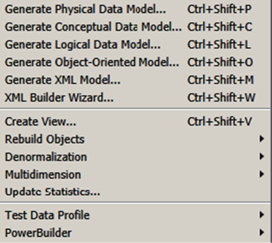
The Tools menu for the PDM is considerably bigger than that for the CDM and LDM. Figure 17.21 shows the central part of the menu; everything above and below this point is shared with the other models.
You can generate five different types of models from a PDM; for the XML model, you have a choice of two mechanisms.
There is a wizard for creating Views, which we’ll show you shortly. The Rebuild options enable to you make sure your indexes, primary keys, references, procedures, and packages are correct. The Denormalization options enable you to transform your model to improve performance. You can connect to a database to update the database statistics in the model. You can import or export test data profiles, for use when generating test data (see the Database menu). The Multidimension options allow you to convert a standard PDM into a data warehouse PDM, and rebuild Cubes  . Finally, you can communicate with PowerBuilder to exchange metadata, which enables you to refactor existing PowerBuilder applications within PowerDesigner.
Most of the preceding topics are beyond the ‘made simple’ label of this book.
Figure 17.21 The PDM tools menu
Approaches for Creating a PDM
You can use a variety of techniques to create a PDM in PowerDesigner. Which approach is appropriate for you will depend on the models and information you have available.
· Create from scratch
· Generate a PDM from a SAM (CDM) or another PDM
· Generate a PDM from a LDM
· Copy or replicate tables, etc. from other PDMs, including reference models held in the Library
· Use the Excel Import facility to create or update objects in your PDM
The Physical Diagram Palette
Figure 17.22 shows the Toolbox dedicated to physical diagram symbols. The tools on this palette allow you to create or select (from left to right):
Packages |
|
Tables | |
Views | |
References | |
Procedures | |
Files |


The procedures tool is unavailable in this palette, because the current DBMS does not support procedures.
Creating a Reference from the Palette
A reference in the PDM is drawn in the opposite direction from what you are used to in the CDM and LDM. To draw a reference, click on the reference tool in the palette, click on the child table first, then click on the parent. Think of it as drawing a line from one table to another table that it references, or needs data from.
Reference Optionality & Cardinalities
In the CDM and LDM, you adjust the relationship optionality and cardinalities in one place, the relationship’s ‘Cardinalities’ tab.
In the PDM, you change the optionality of the parent table in a reference by adjusting the optionality of the foreign key column in the child table. The child cardinalities are adjusted via the ‘Integrity’ tab on the reference property sheet.
 The reference name is not the same as the name of the foreign key constraint; this is on the reference’s ‘Integrity’ tab.
![]() “Reference Properties” (Data Modeling)
“Reference Properties” (Data Modeling)
Creating a View
There are several ways to create a view. Here is the simplest and quickest way:
1. In the Browser or diagram, select the tables, views, and references that the new view needs to include.
2. Select Tools|Create View menu to create the view.
a. PowerDesigner will automatically create the required SQL, including WHERE clauses (if you selected the necessary references).
b. The ‘Columns’ tab on the view property sheet shows a list of all the table columns and view columns in the query.
c. This list cannot be edited – edit the query (on the ‘SQL Query’ tab), instead.
d. Dependencies are automatically created between the view and the tables, and between the view columns and table columns. These can be seen on the object ‘Dependencies’ tabs.
3. Tailor the SQL to remove unwanted columns and refine the logic.
4. On the diagram, draw traceability links to show dependencies.
For example, I selected the tables and reference in Figure 17.23, and the ‘create view’ wizard automatically created the view called View_1. PowerDesigner will not create any diagrammatic links between the tables and the view; you can add these yourself if you want.
Figure 17.23 A wizard view

Figure 17.24 shows the SQL Query generated by PowerDesigner.
Figure 17.24 The SQL query

Using the tools in this tab, you can edit the Query using a built-in SQL editor or an external editor.
Display Preferences
The PDM Display Preferences are fundamentally the same as you have already seen, with a different list of object types.
SQL Preview
PowerDesigner allows you to preview the code that will be generated for an object, even for the whole PDM. Figure 17.25 shows the preview for a table. The tools on the toolbar allow you to choose the parts of the SQL to include.
Figure 17.25 SQL Preview

![]() “Previewing SQL Statements” (Data Modeling)
“Previewing SQL Statements” (Data Modeling)
Viewing Data
Right-click a table in the Browser or diagram and select View Data. This allows you to connect to a database and look at the data in the table.
Denormalization in PowerDesigner
 PowerDesigner supports all five of the denormalization techniques described in this chapter. Table 17.5 summarizes how that support is provided. In addition, PowerDesigner supports Horizontal and Vertical Partitioning of tables.
All of the denormalization techniques are available via the Tools menu, and also via the contextual menu for tables. When you run one of these processes, you have the option to retain the original tables. It is always advisable to do this, for several reasons:
· To preserve generation dependencies and other links in the original tables
· PowerDesigner links the original and new tables; these links are accessible via the ‘Version Info’ tab
· Some of the transformation definitions can be altered, allowing you to experiment with alternative design approaches
o For example, re-arranging the columns in a vertical partition
· The Generate property can be set to ‘false’ in the original tables, preventing them from being generated in future models or database schemas
Assuming the PDM was generated from another model, retaining the original tables improves the update process, should you update the PDM via the ‘generation’ feature.
Table 17.5 Denormalization in PowerDesigner
Technique | Approach |
Standard | The ‘Table Collapsing’ feature. |
FUBES | The ‘Column Denormalization’ feature. Alternatively, replicate columns with the standard replication feature, although this will not appear in the list of model transformations. |
Repeating Groups | Replicate columns with the standard replication feature – this will not appear in the list of model transformations. |
Repeating Data Elements | The ‘Column Denormalization’ feature. |
Summarization | Create a new summary table. To create similar tables, either copy or replicate the original. |
Star Schema | Combine the FUBES and Repeating Data Element Techniques. |
The denormalization features work in pretty much identical fashion - you choose one or more tables to work with, then tell PowerDesigner what to do with them. You can experiment with this in Exercise 21. The results of each denormalization process are stored in the model as Transformations, and a list of them is available from the Model menu. See Figure 17.26.
Figure 17.26 List of transformations

For example, assume that the column ICE_CREAM_CONTAINER.HEIGHT has been denormalized into the ICE_CREAM_SALES table. Figure 17.27 shows part of the ‘version info’ for the denormalized column. This allows you to access the details of the transformation (and hence the original object), and to break the link back to the original object.
Figure 17.27 Link back to the original
![]()
Figure 17.28 shows the impact analysis for the original column, with the link to the new column.
Figure 17.28 Link to the new column

Collapsing Subtypes
There is one more way of denormalizing a model where the LDM has an inheritance structure. For example, consider the structure in Figure 16.1, reproduced here as Figure 17.29.
Figure 17.29 Simple subtypes

In the PDM, we may wish to collapse this structure, and migrate all of the columns in Ice Cream Container to the Cone and Cup tables. The best place to do this is in the LDM, via the ‘Generation’ tab in the Inheritance’s property sheet – uncheck ‘Generate parent’, and ensure that ‘Inherit all attributes’ is selected. Now re-generate the PDM in update mode.
![]() “Denormalizing Tables and Columns” (Data Modeling)
“Denormalizing Tables and Columns” (Data Modeling)
Reverse-engineering Databases
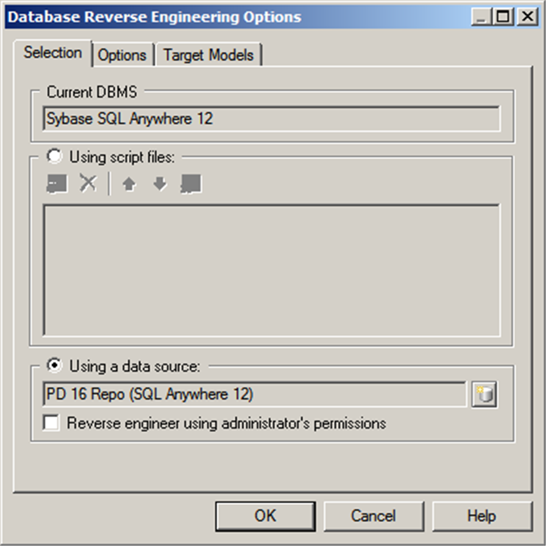
The term ‘reverse-engineering’ refers to the creation of a new PDM by scanning the structure of a database schema or reading SQL scripts. To start the process, select Reverse Engineer|Database on the File menu, and the dialog shown in Figure 17.30 will appear. Type the name of the new model, choose your DBMS, choose any model extension required, and then click on <OK>.
Figure 17.30 Choosing the DBMS etc

Now you have to tell PowerDesigner more about what you want it to do. Where will it find the database definition? Are there any data models open in the workspace representing databases linked to the one you’re reverse-engineering? Provide some detailed options, such as whether or not you want diagram symbols created in the new model. In Figure 17.31, I want to create a PDM by reverse-engineering the structure of my PowerDesigner repository database.
PowerDesigner will read the source material and create the model for you. You can monitor progress in the PowerDesigner Output window.
Remember to save the model in a file, PowerDesigner leaves that up to you.
For some databases (e.g. Microsoft Access), you will need to check DBMS-specific help for detailed instructions on reverse-engineering.
![]() “Reverse Engineering a Database into a PDM” (Data Modeling)
“Reverse Engineering a Database into a PDM” (Data Modeling)
Figure 17.31 Reverse-engineering options
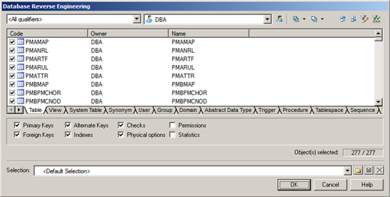
Now you have to choose the database objects that you want to reverse-engineer, using the dialog in Figure 17.32.
Figure 17.32 Choosing your objects
Keeping the Model and Database Synchronized
Okay, you have a database, and you have a PDM. How do you update one from the other? The answer lies in two commands on the Database menu:
Update Model from Database | This uses the same process we showed you for reverse-engineering a database; the model is updated to match the database. If you need to compare a PDM to the current database, compare it with a new PDM you create by reverse-engineering the database. |
Generate Database | Allows you to update a database from a model, either by generating SQL scripts, or by a live connection. Just complete the options listed in Figure 17.33, and click <OK>. |
Figure 17.33 Database generation options

EXERCISE 20: Getting Physical with Subtypes in PowerDesigner
Subtyping is a powerful communication tool on the logical data model, because it allows the modeler to represent the similarities that exist between distinct business concepts to improve integration and data quality. As an example, refer to Figure 17.34, where the supertype Course contains the common data elements and relationships for the Lecture and Workshop subtypes.
Figure 17.34 Course subtyping structure

Briefly walking through this model, we learn that each Course, such as “Data Modeling 101”, can be either a Lecture or a Workshop. Each Course must be taught at many Locations. Each Learning Track, such as the Data Track, must consist of one or many Lectures, yet only one Workshop. Each Workshop, such as the Advanced Design Workshop, can require certain Courses as a prerequisite, such as Data Modeling 101 and Data Modeling 101 Workshop. Each System Administrator must administer one or many Workshops.
Assume this is a logical data model (with data elements hidden to keep this example manageable). On the physical data model, we can replace this subtype symbol in one of three ways:
· Rolling down. Remove the supertype entity and copy all of the data elements and relationships from the supertype to each of the subtypes.
· Rolling up. Remove the subtypes and copy all of the data elements and relationships from each subtype to the supertype. Also add a type code to distinguish the subtypes.
· Identity. Convert the subtype symbol into a series of one-to-one relationships, connecting the supertype to each of the subtypes.
For this Challenge, using the Course structure from Figure 17.34, build all three options.
In PowerDesigner, create a new project for the exercise, then create an initial LDM. Now generate three LDMs from the initial LDM, using the default options. You’ll find the Generate Logical Data Model command on the Tools menu. Use the phrases ‘IDENTITY’, ‘ROLLING DOWN’, and ‘ROLLING UP’ in the model names. Remember that denormalizing subtype structures can only be done in the LDM.
Generate a PDM from each LDM using your choice of DBMS; use the generic ‘ODBC’ option if you like. In each model, carry out the appropriate denormalization manually. See the Appendix for my answers.
EXERCISE 21: Denormalizing a PDM in PowerDesigner
Open the LDM you created in Exercise 18, illustrated in Figure 17.35. Your task is to denormalize this model several different ways, using the techniques described earlier in this chapter. I know we haven’t provided much information about how to run the denormalization features - that is intentional. It’s time for you to do some investigation of the Tools menu. Select the tables you need to denormalize, then select Denormalization on the Tools menu, and select the required technique.
Generate three different PDMs from the LDM, and denormalize them to produce the target models listed in Table 17.6.
Table 17.6 Your tasks
Model Name | Target Model |
Exercise 21 – Identity | See Figure 17.2 |
Exercise 21 – Rolling Down | See Figure 17.3 |
Exercise 21 – Rolling Up | See Figure 17.4 |
Use the phrases ‘IDENTITY’, ‘ROLLING DOWN’, and ‘ROLLING UP’ in the model names.
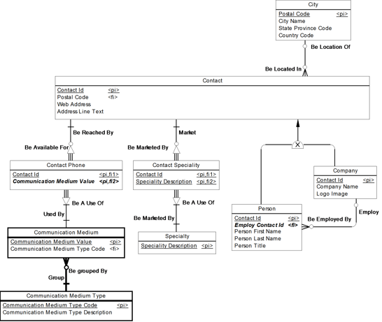
Figure 17.35 Contact data model with Communication Medium
Key Points · The physical data model builds upon the logical data model to produce a technical solution. · Denormalization is the process of selectively violating normalization rules and reintroducing redundancy into the model. · There are five denormalization techniques: standard, repeating groups, repeating data elements, FUBES, and summarization. · A star schema is when each set of tables that make up a dimension is flattened into a single table. · A view is a virtual table. · An index is a pointer to something that needs to be retrieved. · Partitioning is breaking up a table into rows, columns, or both. If a table is broken up into columns, the partitioning is vertical. If a table is broken into rows, the partitioning is horizontal. · Snowflaking is when vertical partitioning is performed on a dimensional model, often due to data volatility or frequent user access to higher levels in a hierarchy. · Data values change over time. We have the option of storing only the new information (Type 1), storing all of the new information plus all of the historical information (Type 2), or storing the new information plus some of the historical information (Type 3). · PowerDesigner does not use object names when generating a database – it uses the object ‘codes’. · When denormalizing, keep the original tables, and uncheck ‘generate’. · The ‘Dependencies’ tab tells you everything about how a column is used. |