1
Characteristics of Human Vision
Stefan Winkler
1.4.1 Lateral Geniculate Nucleus
1.4.3 Multichannel Organization
1.5.3 Contrast Sensitivity Functions
1.7.3 Color Spaces and Conversions
1.1 Introduction
Vision is perhaps the most essential of human senses. A large part of human brain is devoted to vision, which explains the enormous complexity of the human visual system. The human visual system can be subdivided into two major components: the eyes, which capture light and convert it into signals that can be understood by the nervous system, and the visual pathways in the brain, along which these signals are transmitted and processed. This chapter discusses the anatomy and physiology of these components as well as a number of phenomena of visual perception that are of particular relevance to digital imaging.
The chapter is organized as follows. Section 1.2 presents the optics and mechanics of the eye. Section 1.3 discusses the properties and the functionality of the receptors and neurons in the retina. Section 1.4 explains the visual pathways in the brain and a number of components along the way. Section 1.5 reviews human sensitivity to light and various related mathematical models. Section 1.6 discusses the processes of masking and adaptation. Section 1.7 describes the representation of color in the visual system and other useful color spaces. Section 1.8 briefly outlines the basics of depth perception. Section 1.9 provides conclusions and pointers for further reading.
1.2 Eye
1.2.1 Physical Principles
From an optical point of view, the eye is the equivalent of a photographic camera. It comprises a system of lenses and a variable aperture to focus images on the light-sensitive retina. This section summarizes the optical principles of image formation.
The optics of the eye rely on the physical principles of refraction. Refraction is the bending of light rays at the angulated interface of two transparent media with different refractive indices. The refractive index n of a material is the ratio of the speed of light in vacuum c0 to the speed of light in this material c, that is, n = c0/c. The degree of refraction depends on the ratio of the refractive indices of the two media as well as the angle ϕ between the incident light ray and the interface normal, resulting in n1 sin ϕ1 = n2 sin ϕ2. This is known as Snell’s law.
Lenses exploit refraction to converge or diverge light, depending on their shape. Parallel rays of light are bent outward when passing through a concave lens and inward when passing through a convex lens. These focusing properties of a convex lens can be used for image formation. Because of the nature of the projection, the image produced by the lens is rotated 180° about the optical axis.
Objects at different distances from a convex lens are focused at different distances behind the lens. In a first approximation, this is described by the Gaussian lens formula:
1ds+1di=1f,(1.1)
where ds is the distance between the source and the lens, di is the distance between the image and the lens, and f is the focal length of the lens. An infinitely distant object is focused at focal length, resulting in di = f. The reciprocal of the focal length is a measure of the optical power of a lens, that is, how strongly incoming rays are bent. The optical power is defined as 1m/f and is specified in diopters.
Most optical imaging systems comprise a variable aperture, which allows them to adapt to different light levels. Apart from limiting the amount of light entering the system, the aperture size also influences the depth of field, that is, the range of distances over which objects will appear in focus on the imaging plane. A small aperture produces images with a large depth of field and vice versa. Another side effect of an aperture is diffraction, which is the scattering of light that occurs when the extent of a light wave is limited. The result is a blurred image. The amount of blurring depends on the dimensions of the aperture in relation to the wavelength of the light.
Distance-independent specifications are often used in optics. The visual angle α = 2arctan(s/2D) measures the extent covered by an image of size s at distance D from the eye. Likewise, resolution or spatial frequency are measured in cycles per degree (cpd) of visual angle.
1.2.2 Optics of the Eye
Attempts to make general statements about the eye’s optical characteristics are complicated by the fact that there are considerable variations between individuals. Furthermore, its components undergo continuous changes throughout life. Therefore, the figures given in the following can only be approximations.
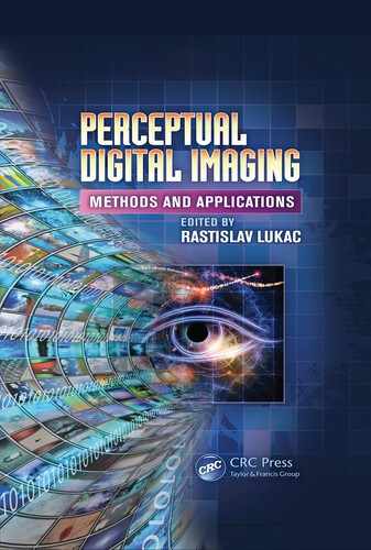
The optical system of the human eye is composed of the cornea, the aqueous humor, the lens, and the vitreous humor, as illustrated in Figure 1.1. The refractive indices of these four components are 1.38, 1.33, 1.40, and 1.34, respectively [1]. The total optical power of the eye is approximately 60 diopters. Most of it is provided by the air-cornea transition, where the largest difference in refractive indices occurs (the refractive index of air is close to 1). The lens itself provides only a third of the total refractive power due to the optically similar characteristics of the surrounding elements.
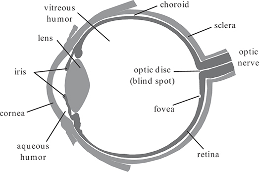
FIGURE 1.1
The human eye (transverse section of the left eye).
The lens is important because its curvature and thus its optical power can be voluntarily increased by contracting muscles attached to it. This process is called accommodation. Accommodation is essential to bringing objects at different distances into focus on the retina. In young children, the optical power of the lens can extend from 20 to 34 diopters. However, this accommodation ability decreases gradually with age until it is lost almost completely, a condition known as presbyopia.
Just before entering the lens, the light passes the pupil, the eye’s aperture. The pupil is the circular opening inside the iris, a set of muscles that control its size and thus the amount of light entering the eye depending on the exterior light levels. Incidentally, the pigmentation of the iris is also responsible for the color of the eyes. The diameter of the pupillary aperture can be varied between 1.5 and 8 mm, corresponding to a thirtyfold change of the quantity of light entering the eye. The pupil is thus one of the mechanisms of the human visual system for light adaptation, which is discussed in Section 1.5.1.
1.2.3 Optical Quality
The physical principles described in Section 1.2.1 pertain to an ideal optical system, whose resolution is only limited by diffraction. While the parameters of an individual healthy eye are usually correlated in such a way that the eye can produce a sharp image of a distant object on the retina, imperfections in the lens system can introduce additional distortions that affect image quality. In general, the optical quality of the eye deteriorates with increasing distance from the optical axis. This is not a severe problem, however, because visual acuity also decreases there, as will be discussed in Section 1.3.
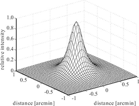
FIGURE 1.2
Point spread function of the human eye as a function of visual angle [3].
The blurring introduced by the eye’s optics can be measured [2] and quantified by the point spread function (PSF) or line spread function of the eye, which represent the retinal images of a point or thin line, respectively; their Fourier transform is the modulation transfer function. A simple approximation of the foveal PSF of the human eye according to Reference [3] is shown in Figure 1.2 for a pupil diameter of 4 mm. The amount of blurring depends on the pupil size. Namely, for small pupil diameters up to 3 or 4 mm, the optical blurring is close to the diffraction limit; as the pupil diameter increases (for lower ambient light intensities), the width of the PSF increases as well, because the distortions due to cornea and lens imperfections become large compared to diffraction effects [4]. The pupil size also determines the depth of field.
FIGURE 1.3
Variation of the modulation transfer function of a human eye model with wavelength [5].
Because the cornea is not perfectly symmetric, the optical properties of the eye are orientation dependent. Therefore, it is impossible to perfectly focus stimuli of all orientations simultaneously, a condition known as astigmatism. This results in a point spread function that is not circularly symmetric. Astigmatism can be severe enough to interfere with perception, in which case it has to be corrected by compensatory glasses.
The properties of the eye’s optics, most important the refractive indices of the optical elements, also vary with wavelength. This means that it is impossible to focus all wavelengths simultaneously, an effect known as chromatic aberration. The point spread function thus changes with wavelength. Chromatic aberration can be quantified by determining the modulation transfer function of the human eye for different wavelengths. This is shown in Figure 1.3 for a human eye model with a pupil diameter of 3 mm and in focus at 580 nm [5]. It is evident that the retinal image contains only poor spatial detail at wavelengths far from the in-focus wavelength (note the sharp cutoff going down to a few cycles per degree at short wavelengths). This tendency toward monochromacy becomes even more pronounced with increasing pupil aperture.
1.2.4 Eye Movements
The eye is attached to the head by three pairs of muscles that provide for rotation around its three axes. Several different types of eye movements can be distinguished [6]. Fixation movements are perhaps the most important. The voluntary fixation mechanism allows to direct the eyes toward an object of interest. This is achieved by means of saccades, high-speed movements steering the eyes to the new position. Saccades occur at a rate of two to three per second and are also used to keep scanning the entire scene by fixating on one highlight after the other. One is unaware of these movements because the visual image is suppressed during saccades. The involuntary fixation mechanism locks the eyes on the object of interest once it has been found. It involves so-called micro-saccades that counter the tremor and slow drift of the eye muscles. The same mechanism also compensates for head movements or vibrations.
Additionally, the eyes can track an object that is moving across the scene. These so-called pursuit movements can adapt to object trajectories with great accuracy. Smooth pursuit works well even for high velocities, but it is impeded by large accelerations and unpredictable motion.
Understanding what drives the eye movements, or in other words, why people look at certain areas in an image, has been an intriguing problem in vision research for a long time. It is important for perceptual imaging applications since visual acuity of the human eye is not uniform across the entire visual field. In general, visual acuity is highest only in a relatively small cone around the optical axis (the direction of gaze) and decreases with distance from the center. This is due to the deterioration of the optical quality of the eye toward the periphery (see above) as well as the layout of the retina (see Section 1.3).
Experiments presented in Reference [7] demonstrated that the saccadic patterns depend on the visual scene as well as the cognitive task to be performed. The direction of gaze is not completely idiosyncratic to individual viewers; however, a significant number of viewers will focus on the same regions of a scene [8], [9]. These experiments have given rise to various theories regarding the pattern of eye movements. Salient points attracting attention is a popular hypothesis [10], which is appealing in passive viewing conditions, such as when watching television. Salient locations of the image are based on local image characteristics, such as color, intensity, contrast, orientation, motion, etc. However, because this hypothesis is purely stimulus driven, it has limited applicability in real life, where semantic content rather than visual saliency drives eye movements during visual search [11]. There are also information-theoretic models that attempt to explain the pattern of eye movements [12].
1.3 Retina
The optics of the eye project images of the outside world onto the retina, the neural tissue at the back of the eye. The functional components of the retina are illustrated in Figure 1.4. Light entering the retina has to traverse several layers of neurons before it reaches the light-sensitive layer of photoreceptors and is finally absorbed in the pigment layer. The anatomy and physiology of the photoreceptors and the retinal neurons is discussed in more detail below.
1.3.1 Photoreceptors
The photoreceptors are specialized neurons that make use of light-sensitive photochemicals to convert the incident light energy into signals that can be interpreted by the brain. There are two different types of photoreceptors, namely, rods and cones. The names are derived from the physical appearance of their light-sensitive outer segments (Figure 1.4). Rods are responsible for scotopic vision at low light levels, while cones are responsible for photopic vision at high light levels.
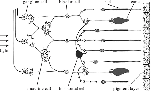
FIGURE 1.4
Anatomy of the retina. © 1991 W.B. Saunders
Rods are very sensitive light detectors. With the help of the photochemical rhodopsin, they can generate a photocurrent response from the absorption of only a single photon [13]. However, visual acuity under scotopic conditions is poor, even though rods sample the retina very finely. This is because signals from many rods converge onto a single neuron, which improves sensitivity but reduces resolution.
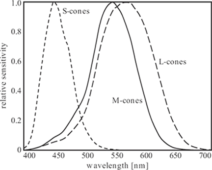
The opposite is true for the cones. Several neurons encode the signal from each cone, which already suggests that cones are important components of visual processing. There are three different types of cones, which can be classified according to the spectral sensitivity of their photochemicals. These three types are referred to as L-, M-, and S-cones, corresponding to their sensitivity to long, medium, and short wavelengths, respectively. Therefore, sometimes cones are also referred to as red, green, and blue cones, respectively. Estimates of the absorption spectra of the three cone types are shown in Figure 1.5 [14], [15], [16]. The peak sensitivities occur around 570 nm, 570 nm, and 440 nm, respectively. As can be seen, the absorption spectra of the L- and M-cones are very similar, whereas the S-cones exhibit a significantly different sensitivity curve. The cones form the basis of color perception. The overlap of the spectra is essential to fine color discrimination (color perception is discussed in more detail in Section 1.7).
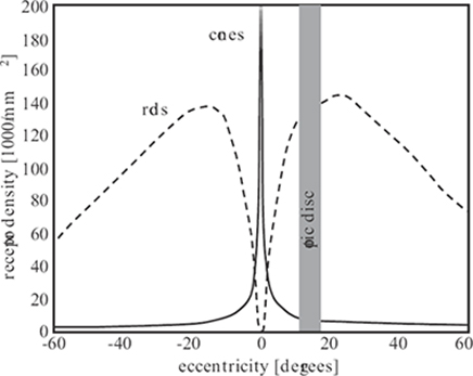
FIGURE 1.6
The distribution of photoreceptors on the retina [17]. Cones are concentrated in the fovea at the center of the retina, whereas rods dominate in the periphery. The gap around 15 degrees eccentricity represents the blind spot around the optic disc, where no receptors are present.
There are approximately 5 million cones and 100 million rods in each eye. Their density varies greatly across the retina, as is evident from Figure 1.6 [17]. There is also a large variability between individuals. Cones are concentrated in the fovea, a small area near the center of the retina, where they can reach a peak density of up to 300,000/mm2 [18]. Throughout the retina, L- and M-cones are in the majority; S-cones are much more sparse and account for less than 10% of the total number of cones [19]. Rods dominate outside of the fovea, which explains why it is easier to see very dim objects (for example, stars) when they are in the peripheral field of vision than when looking straight at them. The central fovea contains no rods at all. The highest rod densities (up to 200,000/mm2) are found along an elliptical ring near the eccentricity of the optic disc. The blind spot around the optic disc, where the optic nerve exits the eye, is completely void of photoreceptors.
The spatial sampling of the retina by the photoreceptors is illustrated in Figure 1.7. In the fovea, the cones are tightly packed and form a hexagonal sampling array. In the periphery, the sampling grid becomes more irregular; the separation between the cones grows, and rods fill in the spaces. Also note the size differences: the cones in the fovea have a diameter of 1 to 3 µm; in the periphery, their diameter increases to 5 to 10 µm. The diameter of the rods varies between 1 and 5 µm.
The size and spacing of the photoreceptors determine the maximum spatial resolution of the human visual system. Assuming an optical power of 60 diopters and thus a focal length of approximately 17 mm for the eye, distances on the retina can be expressed in terms of visual angle using simple trigonometry. The entire fovea covers approximately 2 degrees of visual angle. The L- and M-cones in the fovea are spaced approximately 2.5 µm apart, which corresponds to 30 arc seconds of visual angle. The maximum resolution of around 60 cpd attained here is high enough to capture all of the spatial variation after the blurring by the eye’s optics. S-cones are spaced approximately 50 µm or 10 minutes of arc apart on average, resulting in a maximum resolution of only 3 cpd [19]. This is consistent with the strong defocus of short-wavelength light due to the axial chromatic aberration of the eye’s optics (see Figure 1.3). Thus, the properties of different components of the visual system fit together nicely, as can be expected from an evolutionary system. The optics of the eye set limits on the maximum visual acuity, and the arrangements of the mosaic of the S-cones as well as the L- and M-cones can be understood as a consequence of the optical limitations (and vice versa).
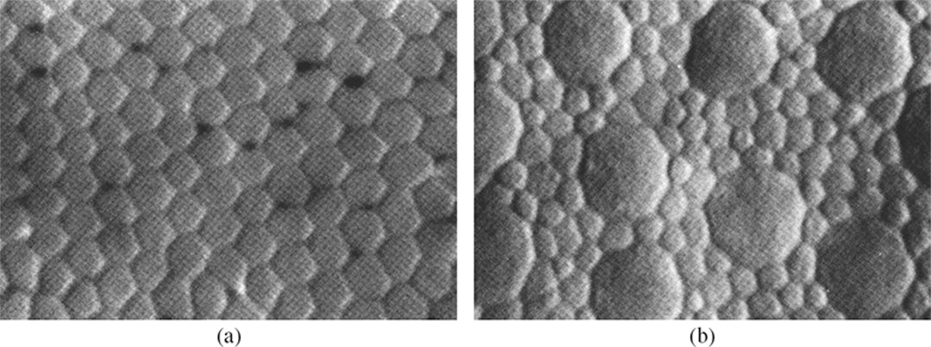
FIGURE 1.7
The photoreceptor mosaic on the retina [17]. (a) In the fovea, the cones are densely packed on a hexagonal sampling array. (b) In the periphery, their size and separation grows, and rods fill in the spaces. Each image shows an area of 35 × 25 µm2. ©1990 John Wiley & Sons
1.3.2 Retinal Neurons
The retinal neurons process the photoreceptor signals. The anatomical connections and neural specializations within the retina combine to communicate different types of information about the visual input to the brain. As shown in Figure 1.4, a variety of different neurons can be distinguished in the retina:
Horizontal cells connect the synaptic nodes of neighboring rods and cones. They have an inhibitory effect on bipolar cells.
Bipolar cells connect horizontal cells, rods, and cones with ganglion cells. Bipolar cells can have either excitatory or inhibitory outputs.
Amacrine cells transmit signals from bipolar cells to ganglion cells or laterally between different neurons. About 30 types of amacrine cells with different functions have been identified.
Ganglion cells collect information from bipolar and amacrine cells. There are about 1.6 million ganglion cells in the retina. Their axons form the optic nerve that leaves the eye through the optic disc and carries the output signal of the retina to other processing centers in the brain (see Section 1.4).
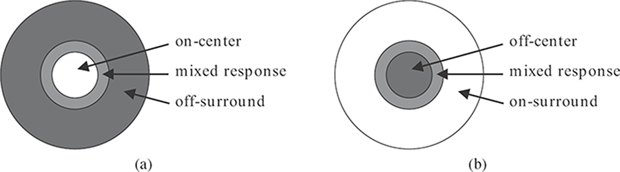
FIGURE 1.8
Center-surround organization of the receptive field of retinal ganglion cells: (a) on-center, off-surround, and (b) off-center, on-surround.
The interconnections between these cells give rise to an important concept in visual perception, the receptive field. The visual receptive field of a neuron is defined as the retinal area in which light influences the neuron’s response. It is not limited to cells in the retina; many neurons in later stages of the visual pathways can also be described by means of their receptive fields (see Sections 1.4.1 and 1.4.2).
The ganglion cells in the retina have a characteristic center-surround receptive field, which is nearly circularly symmetric as shown in Figure 1.8. Light falling directly on the center of a ganglion cell’s receptive field may either excite or inhibit the cell. In the surrounding region, light has the opposite effect. Between center and surround, there is a small area with a mixed response. About half of the retinal ganglion cells have an on-center, off-surround receptive field; that is, they are excited by light on their center. The other half have an off-center, on-surround receptive field with the opposite reaction. This receptive field organization is mainly due to lateral inhibition from horizontal cells. The consequence is that excitatory and inhibitory signals basically neutralize each other when the stimulus is uniform. However, for example, when edges or corners come to lie over such a cell’s receptive field, its response is amplified. In other words, retinal neurons implement a mechanism of contrast computation (see also Section 1.5.4).
Ganglion cells can be further classified in two main groups:
P-cells constitute the large majority (nearly 90%) of ganglion cells. They have very small receptive fields; that is, they receive inputs only from a small area of the retina (only a single cone in the fovea) and can thus encode fine image details. Furthermore, P-cells encode most of the chromatic information as different P-cells respond to different colors.
M-cells constitute only 5 to 10% of ganglion cells. At any given eccentricity, their receptive fields are several times larger than those of P-cells. They also have thicker axons, which means that their output signals travel at higher speeds. M-cells respond to motion or small differences in light level but are insensitive to color. They are responsible for rapidly alerting the visual system to changes in the image.
These two types of ganglion cells represent the origin of two separate visual streams in the brain, the so-called magnocellular and parvocellular pathways (see Section 1.4.1).

FIGURE 1.9
Visual pathways in the human brain. ©1991 W.B. Saunders
As becomes evident from this intricate arrangement of neurons, the retina is much more than a device to convert light to neural signals; the visual information is thoroughly preprocessed here before it is passed on to other parts of the brain.
1.4 Visual Pathways
The optic nerve leaves the eye to carry the visual information from the ganglion cells of the retina to various processing centers in the brain. These visual pathways are illustrated in Figure 1.9. The optic nerves from the two eyes meet at the optic chiasm, where the fibers are rearranged. All the fibers from the nasal halves of each retina cross to the opposite side, where they join the fibers from the temporal halves of the opposite retinas to form the optic tracts. Since the retinal images are reversed by the optics, the left visual field is processed in the right hemisphere, and the right visual field is processed in the left hemisphere.
Most of the fibers from each optic tract synapse in the lateral geniculate nucleus (see Section 1.4.1). From there fibers pass by way of the optic radiation to the visual cortex (see Section 1.4.2). Throughout these visual pathways, the neighborhood relations of the retina are preserved; that is, the input from a certain small part of the retina is processed in a particular area of the lateral geniculate nucleus and of the primary visual cortex. This property is known as retinotopic mapping.
There are a number of additional destinations for visual information in the brain apart from the major visual pathways listed above. These brain areas are responsible mainly for behavioral or reflex responses. One example is the superior colliculus, which seems to be involved in controlling eye movements in response to certain stimuli in the periphery.
1.4.1 Lateral Geniculate Nucleus
The lateral geniculate nucleus comprises around one million neurons in six layers. The two inner layers, the magnocellular layers, receive input almost exclusively from M-type ganglion cells. The four outer layers, the parvocellular layers, receive input mainly from P-type ganglion cells. As mentioned in Section 1.3.2, the M- and P-cells respond to different types of stimuli, namely, motion and spatial detail, respectively. This functional specialization continues in the lateral geniculate nucleus and the visual cortex, which suggests the existence of separate magnocellular and parvocellular pathways in the visual system.
The specialization of cells in the lateral geniculate nucleus is similar to the ganglion cells in the retina. The cells in the magnocellular layers are effectively color-blind and have larger receptive fields. They respond vigorously to moving contours. The cells in the parvocellular layers have rather small receptive fields and are differentially sensitive to color. They are excited if a particular color illuminates the center of their receptive field and inhibited if another color illuminates the surround. Only two color pairings are found, namely, red-green and blue-yellow. These opponent colors form the basis of color perception in the human visual system and will be discussed in more detail in Section 1.7.2.
The lateral geniculate nucleus not only serves as a relay station for signals from the retina to the visual cortex but also controls how much of the information is allowed to pass. This gating operation is controlled by extensive feedback signals from the primary visual cortex as well as input from the reticular activating system in the brain stem, which governs a general level of arousal.
1.4.2 Visual Cortex
The visual cortex is located at the back of the cerebral hemispheres (see Figure 1.9). It is responsible for all higher-level aspects of vision. The signals from the lateral geniculate nucleus arrive at an area called the primary visual cortex (also known as area V1, Brodmann area 17, or striate cortex), which makes up the largest part of the human visual system. In addition to the primary visual cortex, more than 20 other cortical areas receiving strong visual input have been discovered. Little is known about their exact functionalities, however.
There is an enormous variety of cells in the visual cortex. Neurons in the first stage of the primary visual cortex have center-surround receptive fields similar to cells in the retina and in the lateral geniculate nucleus (see above). A recurring property of many cells in the subsequent stages of the visual cortex is their selective sensitivity to certain types of information. A particular cell may respond strongly to patterns of a certain orientation or to motion in a certain direction. Similarly, there are cells tuned to particular frequencies, colors, velocities, etc. This neuronal selectivity is thought to be at the heart of the multichannel organization of human vision, which is discussed in Section 1.4.3.
The foundations of knowledge about cortical receptive fields were laid in References [20] and [21]. Based on physiological studies of cells in the primary visual cortex, several classes of neurons with different specializations were identified.
Simple cells behave in an approximately linear fashion; that is, their responses to complicated shapes can be predicted from their responses to small-spot stimuli. They have receptive fields composed of several parallel elongated excitatory and inhibitory regions, as illustrated in Figure 1.10. In fact, their receptive fields resemble Gabor patterns [22]. Hence, simple cells can be characterized by a particular spatial frequency, orientation, and phase. Serving as an oriented bandpass filter, a simple cell thus responds to a certain, limited range of spatial frequencies and orientations.

FIGURE 1.10
Idealized receptive field of a simple cell in the primary visual cortex.
Complex cells are the most common cells in the primary visual cortex. Like simple cells, they are also orientation-selective, but their receptive field does not exhibit the on- and off-regions of a simple cell; instead, they respond to a properly oriented stimulus anywhere in their receptive field.
A small percentage of complex cells respond well only when a stimulus (still with the proper orientation) moves across their receptive field in a certain direction. These direction-selective cells receive input mainly from the magnocellular pathway and probably play an important role in motion perception. Some cells respond only to oriented stimuli of a certain size. They are referred to as end-stopped cells. They are sensitive to corners, curvature, or sudden breaks in lines. Both simple and complex cells can also be end-stopped. Furthermore, the primary visual cortex is the first stage in the visual pathways where individual neurons have binocular receptive fields; that is, they receive inputs from both eyes, thereby forming the basis for stereopsis and depth perception.
1.4.3 Multichannel Organization
As mentioned above, many neurons in the visual system are tuned to certain types of visual information, such as color, frequency, and orientation. Data from experiments on pattern discrimination, masking, and adaptation (see Section 1.6) yield further evidence that these stimulus characteristics are processed in different channels in the human visual system. This empirical evidence motivated the multichannel theory of human vision, which provides an important framework for understanding and modeling pattern sensitivity.
A large number of neurons in the primary visual cortex have receptive fields that resemble Gabor patterns (Figure 1.10). Hence, they can be characterized by a particular spatial frequency and orientation, and essentially represent oriented bandpass filters. There is still a lot of discussion about the exact tuning shape and bandwidth, and different experiments have led to different results. For the achromatic visual pathways, most studies give estimates of approximately one to two octaves for the spatial frequency bandwidth and 20 to 60 degrees for the orientation bandwidth, varying with spatial frequency [23]. These results are confirmed by psychophysical evidence from studies of discrimination and interaction phenomena. Interestingly, these cell properties can also be related with and even derived from the statistics of natural images [24], [25].
Fewer empirical data are available for the chromatic pathways. They probably have similar spatial frequency bandwidths [26], [27], whereas their orientation bandwidths have been found to be significantly larger, ranging from 60 to 130 degrees [28].
Many different transforms and filters have been proposed as approximations to the multichannel representation of visual information in the human visual system. These include Gabor filters (Figure 1.10), the Cortex transform [29], a variety of wavelets, and the steerable pyramid [30]. While the specific filter shapes and designs are very different, they all decompose an image into a number of spatial frequency and orientation bands. With a sufficient number of appropriately tuned filters, all stimulus orientations and frequencies in the sensitivity range of the visual system can be covered.
1.5 Sensitivity to Light
1.5.1 Light Adaptation
The human visual system is capable of adapting to an enormous range of light intensities. Light adaptation allows to better discriminate relative luminance variations at every light level. Scotopic and photopic vision together cover twelve orders of luminance magnitude, from the detection of a few photons to vision in bright sunlight. However, at any given level of adaptation, humans only respond to an intensity range of two to three orders of magnitude. Three mechanisms for light adaptation can be distinguished in the human visual system:
The mechanical variation of the pupillary aperture. As discussed in Section 1.2.2, it is controlled by the iris. The pupil diameter can be varied between 1.5 and 8 mm, which corresponds to a thirtyfold change of the quantity of light entering the eye. This adaptation mechanism responds in a matter of seconds.
The chemical processes in the photoreceptors. This adaptation mechanism exists in both rods and cones. In bright light, the concentration of photochemicals in the receptors decreases, thereby reducing their sensitivity. On the other hand, when the light intensity is reduced, the production of photochemicals and thus the receptor sensitivity is increased. While this chemical adaptation mechanism is very powerful (it covers five to six orders of magnitude), it is rather slow; complete dark adaptation in particular can take up to an hour.
Adaptation at the neural level. This mechanism involves neurons in all layers of the retina, which adapt to changing light intensities by increasing or decreasing their signal output accordingly. Neural adaptation is less powerful, but faster than the chemical adaptation in the photoreceptors.
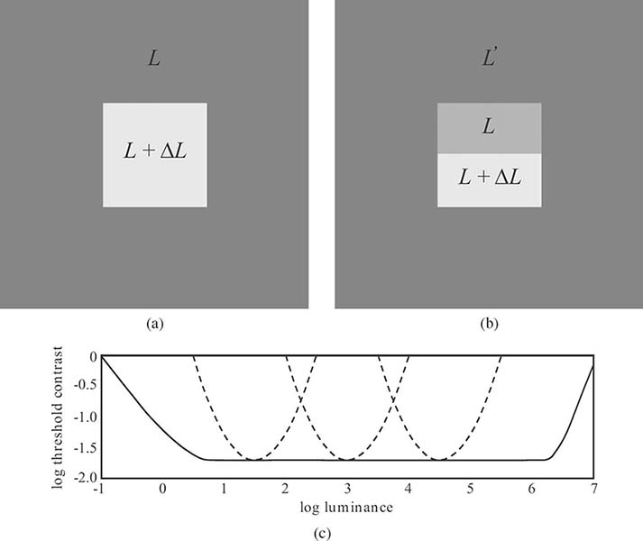
FIGURE 1.11
Illustration of the Weber-Fechner law. Using the basic stimulus shown in (a), threshold contrast is constant over a wide range – shown as a solid line in (c). When the adapting luminance L′ is different from L as shown in (b), this contrast constancy is lost – shown as dotted lines for various L′ in (c).
1.5.2 Contrast Sensitivity
The response of the human visual system depends much less on the absolute luminance than on the relation of its local variations to the surrounding luminance. This property is known as the Weber-Fechner law. Contrast is a measure of this relative variation of luminance. Mathematically, Weber contrast can be expressed as
CW=ΔLL.(1.2)
This definition is most appropriate for patterns consisting of a single increment or decrement ΔL to an otherwise uniform background luminance.
The threshold contrast, which is the minimum contrast necessary for an observer to detect a change in intensity, is shown as a function of background luminance in Figure 1.11. As can be seen, it remains nearly constant over an important range of intensities (from faint lighting to daylight) due to the adaptation capabilities of the human visual system, that is, the Weber-Fechner law holds in this range. This is indeed the luminance range typically encountered in most image processing applications. Outside of this range, intensity discrimination ability of the human eye deteriorates. Under optimal conditions, the threshold contrast can be less than 1%. The exact figure depends greatly on the stimulus characteristics, most important, its color and spatial frequency (see Section 1.5.3).

FIGURE 1.12
Sinusoidal grating with Michelson contrast of CM = 0.6 and its luminance profile.
The Weber-Fechner law is only an approximation of the actual sensory perception. Most important, it presumes that the visual system is adapted to the background luminance L. This assumption is generally violated when looking at a natural image in print or on screen. If the adapting luminance L′ is different, as depicted in Figure 1.11b, the required threshold contrast can become much larger, depending on how far L and L′ are apart. Even this latter scenario is a simplification of realistic image viewing situations, because the adaptation state is determined not only by the environment, but also by the image content itself. Besides, most images are composed of many more than just two colors, so the response of the visual system becomes much more complex.
1.5.3 Contrast Sensitivity Functions
The dependencies of threshold contrast on stimulus characteristics can be quantified using contrast sensitivity functions (CSFs); contrast sensitivity is simply the inverse of the contrast threshold. In these CSF measurements, the contrast of periodic (often sinusoidal) stimuli with varying frequencies is defined as the Michelson contrast:
CM=Lmax−LminLmax+Lmin,(1.3)
where Lmin and Lmax are the luminance extrema of the pattern (see Figure 1.12).
CSF approximations to measurements from Reference [31] are shown in Figure 1.13. Achromatic contrast sensitivity is generally higher than chromatic, especially at high spatial frequencies. This is the justification for chroma subsampling in image compression applications; for example, humans are relatively insensitive to a reduction of color detail. Achromatic sensitivity has a distinct maximum around 2 to 8 cpd (again depending on stimulus characteristics) and decreases at low spatial frequencies,1 whereas chromatic sensitivity does not. The chromatic CSFs for red-green and blue-yellow stimuli are very similar in shape; the blue-yellow sensitivity is slightly lower overall, and its high-frequency decline sets in a bit earlier.
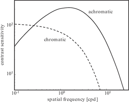
FIGURE 1.13
Approximations of achromatic and chromatic contrast sensitivity functions to data from Reference [31].
Aside from the pattern and color of the stimulus, the exact shape of the contrast sensitivity function depends on many other factors. Among them are the retinal illuminance [33], which has a substantial effect on the location of the maximum, and the orientation of the stimulus [34] (the sensitivity is highest for horizontal and vertical patterns, whereas it is reduced for oblique stimuli).
Various CSF models have been proposed in the literature. A simple yet effective engineering model that can fit both achromatic and chromatic sensitivity measurements in different situations was suggested in Reference [35]:
CSF(f)=(a0+a1f)ea2fa3,(1.4)
where ai are design parameters. More elaborate models have explicit luminance and orientation parameters [36], [37].
1.5.4 Image Contrast
The two definitions of contrast in Equations 1.2 and 1.3 are not equivalent and do not even share a common range of values: Michelson contrast can range from 0 to 1, whereas Weber contrast can range from − 1 to ¥. While they are good predictors of perceived contrast for simple stimuli, they fail when stimuli become more complex and cover a wider frequency range, for example, Gabor patches [38]. It is also evident that none of these simple global definitions are appropriate for measuring contrast in natural images, since a few very bright or very dark spots would determine the contrast of the whole image. Actual human contrast perception on the other hand varies with the local average luminance.
1This apparent attenuation of sensitivity toward low frequencies may be attributed to implicit masking, that is, masking by the spectrum of the window within which the test gratings are presented [32].
In order to address these issues, Reference [39] proposed a local band-limited contrast that measures incremental or decremental changes with respect to the local background:
CPj[x,y]=ψj*L[x,y]ϕj*L[x,y],(1.5)
where L[x,y] is the luminance image, ψj is a bandpass filter at level j of a filter bank, and ϕj is the corresponding lowpass filter. This definition is analogous to the symmetric (in-phase) responses of vision mechanisms.
However, a complete description of contrast for complex stimuli has to include the antisymmetric (quadrature) responses as well [40]. Analytic filters represent an elegant way to achieve this. The magnitude of the analytic filter response, which is the sum of the energy responses of in-phase and quadrature components, exhibits the desired behavior in that it gives a constant response to sinusoidal gratings.
While the implementation of analytic filters in the one-dimensional case is straightforward, the design of general two-dimensional analytic filters is less obvious because of the difficulties involved when extending the Hilbert transform to two dimensions. Oriented measures of contrast can still be computed, because the Hilbert transform is well defined for filters whose angular support is smaller than π. Such contrast measures are useful for many image processing tasks. They can implement a multichannel representation of low-level vision in accordance with the orientation selectivity of the human visual system (Section 1.4.3) and facilitate modeling aspects, such as contrast sensitivity and pattern masking. They have been used in many vision models and their applications, for example, in perceptual quality assessment of images and video [41]. Using analytic orientation-selective filters ηk[x,y], this oriented contrast can be expressed as:
COjk[x,y]=|ψj∗ηk∗L[x,y]|ϕj∗L[x,y].(1.6)
The design of an isotropic contrast measure is more difficult. As pointed out before, the contrast definition from Equation 1.5 is not suitable because it lacks the quadrature component, and isotropic two-dimensional analytic filters as such do not exist. In order to circumvent this problem, a class of nonseparable filters can be used that generalize the properties of analytic functions in two dimensions. These filters are directional wavelets whose Fourier transform is strictly supported in a convex cone with the apex at the origin. For these filters to have a flat response to sinusoidal stimuli, the angular width of the cone must be strictly less than π. This means that at least three such filters are required to cover all possible orientations uniformly. Using a technique described in Reference [42], such filters can be designed in a very simple and straightforward way; it is even possible to obtain dyadic-oriented decompositions that can be implemented using a filter bank algorithm.
Essentially, this technique assumes K directional wavelets with Fourier transform ˆΨ(r,φ) that satisfy the above requirements and
K−1∑k=0|ˆΨ(r,φ−2πk/K)2|=|ˆψ(r)|2,(1.7)
where ˆψ(r) is the Fourier transform of an isotropic dyadic wavelet. Using these oriented filters, one can define an isotropic contrast measure CIj as the square root of the energy sum of the filter responses, normalized as before by a lowpass band:

FIGURE 1.14
Isotropic local contrast: (a) an example image and (b) its isotropic local contrast CIj[x,y] as given by Equation 1.8.
CIj[x,y]=√2Σk|Ψjk*L[x,y]|2ϕj*L[x,y],(1.8)
where L[x,y] is the input image, and ψjk denotes the wavelet dilated by 2−j and rotated by 2πk/K. The term CIj denotes an orientation- and phase-independent quantity.
Being defined by means of analytic filters it behaves as prescribed with respect to sinusoidal gratings (that is, CIj[x,y]≡CM in this case). This combination of analytic-oriented filters thus produces a meaningful phase-independent isotropic measure of contrast. The example shown in Figure 1.14 demonstrates that it is a very natural measure of local contrast in an image. Isotropy is particularly useful for applications where nondirectional signals in an image are considered [43].
1.5.5 Lightness Perception
Weber’s law already indicates that human perception of brightness, or lightness, is not linear. More precisely, it suggests a logarithmic relationship between luminance and lightness. However, Weber’s law is only based on threshold measurements, and it generally overestimates the sensitivity for higher luminance values. More extensive experiments with tone scales were carried out by Munsell to determine stimuli that are perceptually equidistant in luminance (and also in color). These experiments revealed that a power-law relationship with an exponent of 1/3 is closer to actual perception of lightness. This was standardized by CIE as L* (see Section 1.7.3). A modified log characteristic that can be tuned for various situations with the help of a parameter was proposed in Reference [44]. The different relationships are compared in Figure 1.15.
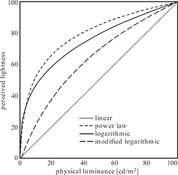
FIGURE 1.15
Perceived lightness as a function of luminance.
1.6 Masking and Adaptation
Masking and adaptation are very important phenomena in vision in general and in digital imaging in particular as they describe interactions between stimuli. Masking occurs when a stimulus that is visible by itself cannot be detected due to the presence of another. As demonstrated in Figure 1.16, the same distortion can be disturbing in certain regions of an image while it is hardly noticeable elsewhere. Thus, within the framework of digital imaging it is helpful to think of features of the processed image being masked by the original image. Results from masking and adaptation experiments were also the basis for developing a multichannel theory of vision (see Section 1.4.3).
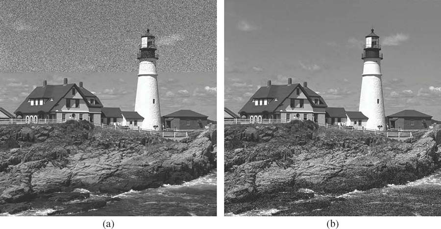
FIGURE 1.16
Demonstration of the masking effect. The same noise has been added to rectangular areas (a) at the top of the image, where it is clearly visible in the sky, and (b) at the bottom of the image, where it is much harder to see on the rocks and in the water due to masking by the heavily textured background.
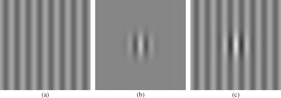
FIGURE 1.17
Typical contrast masking experiment: (a) a cosine masker, (b) a Gabor target, and (c) a superimposed result. The visibility of the target is highly dependent on the contrast of the masker.
1.6.1 Contrast Masking
Spatial masking effects are usually quantified by measuring the detection threshold for a target stimulus when it is superimposed on a masker with varying contrast. The stimuli (both maskers and targets) used in contrast masking experiments are typically sinusoidal gratings or Gabor patches, as shown in Figure 1.17.
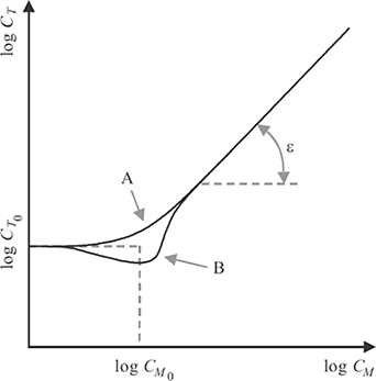
FIGURE 1.18
Illustration of typical masking curves. The detection threshold for the target is elevated by increasing the contrast of the masker. For stimuli with different characteristics, masking is the dominant effect (case A). Facilitation occurs for stimuli with similar characteristics (case B).
Figure 1.18 shows an example of curves approximating the data typically resulting from such experiments. The horizontal axis shows the log of the masker contrast CM, and the vertical axis the log of the target contrast CT at detection threshold. The detection threshold for the target stimulus without any masker is indicated by CT0. For contrast values of the masker larger than CM0, the detection threshold grows exponentially with increasing masker contrast. As can be seen in this figure, case A shows a gradual transition from the threshold range to the masking range. This typically occurs when masker and target have different characteristics. In case B, the detection threshold for the target actually decreases when the masker contrast is close to CM0, which implies that the target is easier to perceive due to the presence of a (weak) masker in this contrast range. This effect is known as facilitation and occurs mainly when target and masker have very similar properties.
The exact masking behavior depends greatly on the types of target and masker stimuli and their relationship to each other (for example, relative frequency and orientation). Masking is strongest when the interacting stimuli have similar characteristics, such as frequencies, orientations, colors, etc. Masking also occurs between stimuli of different orientation [45], between stimuli of different spatial frequency [46], and between chromatic and achromatic stimuli [26], [47], [48], although it is generally weaker.
1.6.2 Pattern Masking
The stimuli (both maskers and targets) used in the experiments cited above are typically sinusoidal gratings or Gabor patches. Compared to natural scene content, they are artificial and quite simplistic. Therefore, masking models based on such experiments do not apply to more complex cases of masking, such as a compression artifact or a watermark in a natural image. Because the observer is not so familiar with the patterns, uncertainty effects become more important, and masking can be much larger.
Not many studies investigate masking in natural images. Reference [49] studied signal detection on complex backgrounds in the presence of noise for medical images and measured defect detectability as a function of signal contrast.
Reference [50] coined the term “entropy masking” to emphasize that the difference between contrast masking with regular structures, such as sinusoidal or Gabor masks on one hand and noise masking (also referred to as texture masking) with unstructured noise-like stimuli on the other, lies mainly in the familiarity of the observer with the stimuli. Natural images are somewhere in between these two extremes.
Reference [51] compared a number of masking models for the visibility of wavelet compression artifacts in natural images. This was one of the first comparative studies of masking in natural images, even if the experiments were quite specific to JPEG2000 encoding. The best results were achieved by a model that considered exclusively the local image activity instead of simple pointwise contrast masking.
Similarly, Reference [52] measured the RMS-based contrast of wavelet distortions at the threshold of visibility in the presence of natural image maskers, which were selected from a texture library. The results were used to parameterize a wavelet-based distortion metric, which was then applied to an associated watermarking algorithm.
Most recently, Reference [53] investigated the visibility of various noise types in natural images. The targets were Gaussian white noise and bandpass filtered noise of varying energy. Psychophysical experiments were conducted to determine the detection threshold of these noise targets on 30 different images with varying content. The achieved results were consistent with data from other masking experiments in a number of ways; namely, detection ability was higher on a plain background, and a clear masking effect was observed. In particular, noise thresholds increase significantly with image activity.
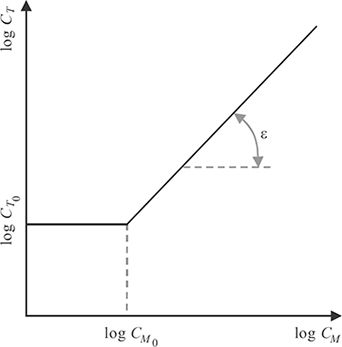
FIGURE 1.19
Simple model of masking given by Equation 1.9.
1.6.3 Masking Models
Numerous masking models of different complexity have been proposed [51], [54]. Because the facilitation effect is usually limited to a rather small and low range of masker contrasts, and because in digital imaging applications, the masker (the image) and the target (the distortions) often have quite different characteristics, facilitation can usually be neglected. The most important effect is clearly masking, that is, the significant increase of the target’s visibility threshold with increasing masker contrast CM. Hence, a simple masking model, shown in Figure 1.19, can be formulated as follows:
CT(CM)={CT0if CM<CM0,CT0(CM/CM0)εotherwise.(1.9)
Other popular masking models in digital imaging are based on contrast gain control, which can explain a wide range of empirical contrast masking data. These models were inspired by analyses of the responses of single neurons in the visual cortex of the cat [55], [56], where contrast gain control serves as a mechanism to keep neural responses within the permissible dynamic range while at the same time retaining global pattern information.
Contrast gain control can be modeled by an excitatory nonlinearity that is inhibited divisively by a pool of responses from other neurons. Masking occurs through the inhibitory effect of the normalizing pool [45], [57]. A further generalization of these models [58] facilitates the integration of channel interactions. Namely, let a = a[c, f, φ, x, y] be a coefficient of the perceptual decomposition in color channel c, frequency band f, orientation band φ, at location [x,y]. Then the corresponding sensor output s = s[c, f, φ, x, y] is computed as
s=αapβ2+h*aq.(1.10)
The excitatory path in the numerator consists of a power-law nonlinearity with exponent p. Its gain is controlled by the inhibitory path in the denominator, which comprises a nonlinearity with exponent q and a saturation constant β to prevent division by zero. The factor a is used to adjust the overall gain of the mechanism.
In the inhibitory path, filter responses are pooled over different channels by means of a convolution with the pooling function h. In its most general form, h = h [c, f, φ, x, y], the pooling operation in the inhibitory path may combine coefficients from the dimensions of color, spatial frequency, orientation, location, and phase.
1.6.4 Pattern Adaptation
Pattern adaptation adjusts the sensitivity of the visual system in response to the prevalent stimulation patterns. For example, adaptation to patterns of a certain frequency can lead to a noticeable decrease of contrast sensitivity around this frequency [59], [60], [61]. Similar in effect to masking, adaptation is a significantly slower process.
An interesting study in this respect was reported in Reference [62]. Natural images of outdoor scenes (both distant views and close-ups) were used as adapting stimuli. It was found that exposure to such stimuli induces pronounced changes in contrast sensitivity. The effects can be characterized by selective losses in sensitivity at lower to medium spatial frequencies. This is consistent with the characteristic amplitude spectra of natural images, which decrease with frequency approximately as 1/f.
Likewise, Reference [63] examined how color sensitivity and appearance might be influenced by adaptation to the color distributions of images. It was found that natural scenes exhibit a limited range of chromatic distributions, so that the range of adaptation states is normally limited as well. However, the variability is large enough so that different adaptation effects may occur for individual scenes or for different viewing conditions.
1.7 Color Perception
In its most general form, light can be described by its spectral power distribution. The human visual system (and most imaging devices for that matter) use a much more compact representation of color, however. This representation and its implications for digital imaging are discussed here.
1.7.1 Color Matching
Color perception can be studied by the color-matching experiment, which is the foundation of color science. In this experiment, the observer views a bipartite field, half of which is illuminated by a test light, the other half by an additive mixture of a certain number of primary lights. The observer is asked to adjust the intensities of the primary lights to match the appearance of the test light.

FIGURE 1.20
CIE XYZ color-matching functions.
It is not a priori clear that it will be possible for the observer to make a match when the number of primaries is small. In general, however, observers are able to establish a match using only three primary lights. This is referred to as the trichromacy of human color vision.2 Trichromacy implies that there exist lights with different spectral power distributions that cannot be distinguished by a human observer. Such physically different lights that produce identical color appearance are called metamers.
As was first established in Reference [64], photopic color matching satisfies homogeneity and superposition and can thus be analyzed using linear systems theory. Assume the test light is known by N samples of its spectral distribution x(λ), expressed as vector x. The color-matching experiment can then be described in matrix form:
t=Cx,(1.11)
where t is a three-dimensional vector whose coefficients are the intensities of the three primary lights found by the observer to visually match x. They are also referred to as the tristimulus coordinates of the test light. The rows of matrix C are made up of N samples of the so-called color-matching functions Ck(λ) of the three primaries.
The Commission Internationale de l’Eclairage (CIE) carried out such color-matching experiments, on the basis of which a two-degree (foveal vision) “standard observer” was defined in 1931. The result was a set of three primaries X, Y, and Z that can be used to match all observable colors by mixing these primaries with positive weights. Y represents the luminance, X and Z are idealized chromaticity primaries. The CIE XYZ color-matching functions are shown in Figure 1.20.
2There are certain qualifications to this empirical generalization that three primaries are sufficient to match any test light. The primary lights must be chosen so that they are visually independent, that is, no additive mixture of any two of the primary lights should be a match to the third. Also, “negative” intensities of a primary must be allowed, which is just a mathematical convention of saying that a primary can be added to the test light instead of to the other primaries.
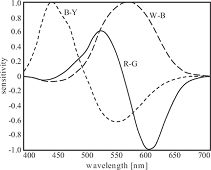
FIGURE 1.21
Normalized spectral sensitivities of white-black (W-B), red-green (R-G), and blue-yellow (B-Y) components of the opponent color space.
The mechanistic explanation of the color-matching experiment is that two lights match if they produce the same absorption rates in the L-, M-, and S-cones. To relate these cone absorption rates to the tristimulus coordinates of the test light, a color-matching experiment is performed with primaries P, whose columns contain N samples of the spectral power distributions of the three primaries Pk(λ). It turns out that the cone absorption rates r are related to the tristimulus coordinates t of the test light by a linear transformation:
r=Mt,(1.12)
where M = RP is a 3 × 3 matrix. This also implies that the color-matching functions are determined by the cone sensitivities up to a linear transformation, which was first verified empirically in Reference [13]. The spectral sensitivities of the three cone types thus provide a satisfactory explanation of the color-matching experiment.
1.7.2 Opponent Colors
Reference [65] was the first to point out that some pairs of hues can coexist in a single color sensation (for example, a reddish yellow is perceived as orange), while others cannot (a reddish green is never perceived, for instance). This led to the conclusion that the sensations of red and green as well as blue and yellow are encoded as color difference signals in separate visual pathways, which is commonly referred to as the theory of opponent colors.
Empirical evidence in support of this theory came from a behavioral experiment designed to quantify opponent colors, the so-called hue cancellation experiment [66]. In this experiment, observers are able to cancel, for example, the reddish appearance of a test light by adding certain amounts of green light. Thus, the red-green or blue-yellow appearance of monochromatic lights can be measured.
Physiological experiments revealed the existence of opponent signals in the visual pathways [67]. It was demonstrated that cones may have an excitatory or an inhibitory effect on ganglion cells in the retina and on cells in the lateral geniculate nucleus. Depending on the cone types, certain excitation/inhibition pairings occur much more often than others: neurons excited by “red” L-cones are usually inhibited by “green” M-cones, and neurons excited by “blue” S-cones are often inhibited by a combination of L- and M-cones. Hence, the receptive fields of these neurons suggest a connection between neural signals and perceptual opponent colors.
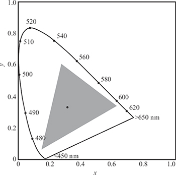
FIGURE 1.22
CIE xy chromaticity diagram. Monochromatic colors, indicated by their wavelengths, along the curve form the border. The dot in the center denotes the location of standard white. The gray triangle represents the gamut of a typical CRT monitor; the color gamut of printers is even smaller.
The reason for an opponent-signal representation of color information in the human visual system may be that the resulting decorrelation of cone signals improves the coding efficiency of the visual pathways. In fact, this representation can also be traced back to the properties of natural image spectra [68]. The spectral sensitivities of an opponent color space derived in Reference [69] are shown in Figure 1.21 as an example. The principal components are white-black (W-B), red-green (R-G), and blue-yellow (B-Y) differences. The W-B channel, which encodes luminance information, is determined mainly by medium to long wavelengths. The R-G channel discriminates between medium and long wavelengths, while the B-Y channel discriminates between short and medium wavelengths.
1.7.3 Color Spaces and Conversions
CIE XYZ color space is very useful as the basis for color conversions because it is device independent. To visualize this color space, chromaticity coordinates are used. The chromaticity coordinates of a color are defined by the normalized weights of the three primaries:
x=XX+Y+Z,y=YX+Y+Z,z=ZX+Y+Z(1.13)
Since by definition x + y + z = 1, the third chromaticity coordinate can now be derived from the first two. All possible sets of tristimulus values can thus be represented in a two-dimensional plot, the so-called chromaticity diagram (Figure 1.22). The monochromatic colors form its border, the spectral locus.
The chromaticity diagram is also used to define color gamuts, which are simply polygons on this diagram. All colors that are additive mixtures of the vertices of a gamut are located inside the gamut. As is evident from the shape of the chromaticity diagram, it is impossible to choose three real primaries such that all possible colors can be matched with additive mixtures of those primaries. The CIE XYZ primaries are actually imaginary. In any real additive color reproductive system such as television, only a limited gamut of colors can be displayed (see Figure 1.22).
An image is typically represented in nonlinear R′G′B′ space to compensate for the behavior of CRT displays (“gamma correction”). For conversion to linear RGB space, each of the resulting three components has to undergo a power-law nonlinearity of the form xγ with γ ≈ 2.5.
RGB space is device dependent, because it is determined by the particular spectral power distribution of the light emitted from the display phosphors. Once the phosphor spectra of the monitor of interest have been determined, the device-independent CIE XYZ tristimulus values can be calculated. The primaries of contemporary monitors are closely approximated by the following transformation [70]:
[XYZ]=[0.412 0.358 0.1800.213 0.715 0.0720.019 0.119 0.950] [RGB].(1.14)
The responses of the L-, M-, and S-cones on the human retina (Section 1.3.1) can then be computed according to Equation 1.12 [71]:
[LMS]=[0.240 0.854 −0.044−0.389 1.160 0.085−0.001 0.002 0.573] [XYZ].(1.15)
The LMS values can be converted to an opponent color space (Section 1.7.2). A variety of opponent color spaces have been proposed, which use different ways to combine the cone responses. The opponent color model from Reference [69] has been designed for maximum pattern-color separability, which has the advantage that color perception and pattern sensitivity can be decoupled. These components are computed from LMS values via the following transformation [69]:
[W−BR−GB−Y]=[0.990−0.106−0.094−0.6690.742−0.027−0.212−0.3540.911] [LMS].(1.16)
One shortcoming of all the above color spaces is their perceptual nonuniformity in terms of color differences. To alleviate this problem, more uniform color spaces were proposed, for example, CIE L*a*b*. It includes a component of perceived lightness (Section 1.5.5) and a color difference equation that is approximately uniform for large color patches. CIE lightness L* is computed according to a power law:3
L*=116(Y/Y0)1/3−16.(1.17)
3Strictly speaking, the power law is only valid when the argument is greater than 0.008856. Below this value, a linear approximation is used due to the singularity of the power function at zero.
The two chromaticity coordinates a* and b* in CIE L*a*b* space are computed as follows:
a*=500[(X/X0)1/3−(Y/Y0)1/3],b*=200[(Y/Y0)1/3−(Z/Z0)1/3],(1.18)
where the 0-subscript refers to the XYZ values of the reference white being used. The CIE L*a*b* color difference is given by
ΔE*ab=√(ΔL*)2+(Δa*)2+(Δb*)2.(1.19)
1.8 Depth Perception
There are a large number of depth cues that the human visual system uses when viewing a three-dimensional scene [72]. These can be classified into oculomotor cues coming from the eye muscles, and visual cues from the scene content itself. They can also be classified into monocular and binocular cues.
Oculomotor cues include accommodation and vergence. As discussed in Section 1.2.2, accommodation refers to the variation of lens shape and thickness (and thus focal length), which allows the eye to focus on an object at a certain distance. Vergence refers to the muscular rotation of the eyeballs, which serves to converge both eyes on the same object.
The visual depth cues also consist of monocular and binocular cues. There are many monocular depth cues, such as:
relative size of objects (close objects usually appear bigger on the retina than the same objects further away),
size of familiar objects,
occlusion (close objects cover parts of objects farther away),
perspective,
texture gradients (the density and perspective of patterns change with distance),
atmospheric blur (objects in the distance appear less sharp because of scatter and turbulence in the atmosphere),
lighting, shading, and shadows, and
motion parallax (when moving, nearby objects cover a larger distance in the field of view than faraway objects).
The most important binocular depth cue is the retinal disparity between points of the same object viewed from slightly different angles by the left and right eye. The resulting apparent displacement of an object viewed along two different lines of sight is called parallax.
Three-dimensional capture and display technology for the digital imaging of scenes with depth rely on (re)producing two or more separate views for the two eyes. An overview of the different technologies can be found in Reference [73]. The separation of the views for processing and display may result in mismatches of various depth cues, which are the main reason for the discomfort many people experience in stereoscopic viewing [74], [75].
1.9 Conclusion
Human vision has intrinsic limitations with respect to the visibility of stimuli, which should be taken into account in digital imaging applications. However, comprehensive modeling of vision processes is made difficult by the sheer complexity of the human visual system. While vision research has produced a large number of models, it has focused mainly on the perception of simple stimuli, such as sinusoids and Gabor patches at threshold; as a result, existing models and data cannot directly be extended to the perception of natural images. This is still very much an active topic of research.
The discussions on human vision in this chapter are necessarily limited in scope; for a more detailed overview, the reader is referred to the abundant literature, such as References [76], [77], and [78].
An exhaustive introduction to optics and vision can be found in Reference [79]. For more details about color science and color perception, the reader is referred to References [80], [81], and [82]. The more specific aspects of image and video quality are addressed in References [41] and [83].
Acknowledgment
This chapter is adapted from Reference [41], with the permission of John Wiley & Sons. Figures 1.4 and 1.9 are adapted from Reference [84]. Figure 1.7 is reprinted from Reference [17], with the permission of John Wiley & Sons.
References
[1] A.C. Guyton and J.E. Hall, Textbook of Medical Physiology. Philadelphia, PA, USA: Saunders, 12th edition, 2010.
[2] D.R. Williams, D.H. Brainard, M.J. McMahon, and R. Navarro, “Double-pass and interferometric measures of the optical quality of the eye,” Journal of the Optical Society of America A, vol. 11, no. 12, pp. 3123–3135, December 1994.
[3] J.K. Ijspeert, T.J. van den Berg, and H. Spekreijse, “An improved mathematical description of the foveal visual point spread function with parameters for age, pupil size and pigmentation,” Vision Research, vol. 33, no. 1, pp. 15–20, January 1993.
[4] J. Rovamo, H. Kukkonen, and J. Mustonen, “Foveal optical modulation transfer function of the human eye at various pupil sizes,” Journal of the Optical Society of America A, vol. 15, no. 9, pp. 2504–2513, September 1998.
[5] D.H. Marimont and B.A. Wandell, “Matching color images: The effects of axial chromatic aberration,” Journal of the Optical Society of America A, vol. 11, no. 12, pp. 3113–3122, December 1994.
[6] R.H.S. Carpenter, Movements of the Eyes. London, UK: Pion, 1988.
[7] A.L. Yarbus, Eye Movements and Vision. New York, USA: Plenum Press, 1967.
[8] L.B. Stelmach and W.J. Tam, “Processing image sequences based on eye movements,” Proceedings of SPIE, vol. 2179, pp. 90–98, February 1994.
[9] C. Endo, T. Asada, H. Haneishi, and Y. Miyake, “Analysis of the eye movements and its applications to image evaluation,” in Proceedings of the Color Imaging Conference, Scottsdale, AZ, USA, November 1994, pp. 153–155.
[10] L. Itti and C. Koch, “A saliency-based search mechanism for overt and covert shifts of visual attention,” Vision Research, vol. 40, no. 10–12, pp. 1489–1506, June 2000.
[11] J.M. Henderson, J.R. Brockmole, M.S. Castelhano, and M. Mack, “Visual saliency does not account for eye movements during visual search in real-world scenes,” in Eye Movements: A Window on Mind and Brain, R. van Gompel, M. Fischer, W. Murray, and R. Hill (eds.), Amsterdam, The Netherlands: Elsevier, 2007, pp. 537–562.
[12] L.W. Renninger, P. Verghese, and J. Coughlan, “Where to look next? Eye movements reduce local uncertainty,” Journal of Vision, vol. 7, no. 3, February 2007.
[13] D.A. Baylor, “Photoreceptor signals and vision,” Investigative Ophthalmology & Visual Science, vol. 28, no. 2, pp. 34–49, January 1987.
[14] A. Stockman, D.I.A. MacLeod, and N.E. Johnson, “Spectral sensitivities of the human cones,” Journal of the Optical Society of America A, vol. 10, no. 12. pp. 2491–2521, December 1993.
[15] A. Stockman, L.T. Sharpe, and C. Fach, “The spectral sensitivity of the human short-wavelength sensitive cones derived from thresholds and color matches,” Vision Research, vol. 39, no. 17, pp. 2901–2927, August 1999.
[16] A. Stockman and L.T. Sharpe, “Spectral sensitivities of the middle- and long-wavelength sensitive cones derived from measurements in observers of known genotype,” Vision Research, vol. 40, no. 13, pp. 1711–1737, June 2000.
[17] C.A. Curcio, K.R. Sloan, R.E. Kalina, and A.E. Hendrickson, “Human photoreceptor topography,” Journal of Comparative Neurology, vol. 292, no. 4, pp. 497–523, February 1990.
[18] P.K. Ahnelt, “The photoreceptor mosaic,” Eye, vol. 12, no. 3B, pp. 531–540, May 1998.
[19] C.A. Curcio, K.A. Allen, K.R. Sloan, C.L. Lerea, J.B. Hurley, I.B. Klock, and A.H. Milam, “Distribution and morphology of human cone photoreceptors stained with anti-blue opsin,” Journal of Comparative Neurology, vol. 312, no. 4, pp. 610–624, October 1991.
[20] D.H. Hubel and T.N. Wiesel, “Receptive fields of single neurons in the cat’s striate cortex,” Journal of Physiology, vol. 148, no. 3, pp. 574–591, October 1959.
[21] D.H. Hubel and T.N. Wiesel, “Receptive fields and functional architecture of monkey striate cortex,” Journal of Physiology, vol. 195, no. 1, pp. 215–243, March 1968.
[22] J.G. Daugman, “Two-dimensional spectral analysis of cortical receptive field profiles,” Vision Research, vol. 20, no. 10, pp. 847–856, October 1980.
[23] G.C. Phillips and H.R. Wilson, “Orientation bandwidth of spatial mechanisms measured by masking,” Journal of the Optical Society of America A, vol. 1, no. 2, pp. 226–232, February 1984.
[24] D.J. Field, “Relations between the statistics of natural images and the response properties of cortical cells,” Journal of the Optical Society of America A, vol. 4, no. 12, pp. 2379–2394, December 1987.
[25] J.H. van Hateren and A. van der Schaaf, “Independent component filters of natural images compared with simple cells in primary visual cortex,” Proceedings of the Royal Society of London B, vol. 265, no. 1394, pp. 1–8, 1998.
[26] M.A. Losada and K.T. Mullen, “The spatial tuning of chromatic mechanisms identified by simultaneous masking,” Vision Research, vol. 34, no. 3, pp. 331–341, February 1994.
[27] M.A. Losada and K.T. Mullen, “Color and luminance spatial tuning estimated by noise masking in the absence of off-frequency looking,” Journal of the Optical Society of America A, vol. 12, no. 2, pp. 250–260, February 1995.
[28] R.L. Pandey Vimal, “Orientation tuning of the spatial-frequency mechanisms of the red-green channel,” Journal of the Optical Society of America A, vol. 14, no. 10, pp. 2622–2632, October 1997.
[29] A.B. Watson, “The cortex transform: Rapid computation of simulated neural images,” Computer Vision, Graphics, and Image Processing, vol. 39, no. 3, pp. 311–327, September 1987.
[30] E.P. Simoncelli, W.T. Freeman, E.H. Adelson, and D.J. Heeger, “Shiftable multi-scale transforms,” IEEE Transactions on Information Theory, vol. 38, no. 2, pp. 587–607, March 1992.
[31] K.T. Mullen, “The contrast sensitivity of human colour vision to red-green and blue-yellow chromatic gratings,” Journal of Physiology, vol. 359, no. 1, pp. 381–400, February 1985.
[32] J. Yang and W. Makous, “Implicit masking constrained by spatial inhomogeneities,” Vision Research, vol. 37, no. 14, pp. 1917–1927, July 1997.
[33] F.L. van Nes and M.A. Bouman, “Spatial modulation transfer in the human eye,” Journal of the Optical Society of America, vol. 57, no. 3, pp. 401–406, March 1967.
[34] M.A. Berkley and F. Kitterle, “Grating visibility as a function of orientation and retinal eccentricity,” Vision Research, vol. 15, no. 2, pp. 239–244, February 1975.
[35] J.L. Mannos and D.J. Sakrison, “The effects of a visual fidelity criterion on the encoding of images,” IEEE Transactions on Information Theory, vol. 20, no. 4, pp. 525–536, July 1974.
[36] P.G.J. Barten, “Evaluation of subjective image quality with the square-root integral method,” Journal of the Optical Society of America A, vol. 7, no. 10, pp. 2024–2031, October 1990.
[37] S. Daly, “The visible differences predictor: An algorithm for the assessment of image fidelity,” in Digital Images and Human Vision, A.B. Watson (ed.), Cambridge, MA, USA: MIT Press, 1993, pp. 179–206.
[38] E. Peli, “In search of a contrast metric: Matching the perceived contrast of Gabor patches at different phases and bandwidths,” Vision Research, vol. 37, no. 23, pp. 3217–3224, December 1997.
[39] E. Peli, “Contrast in complex images,” Journal of the Optical Society of America A, vol. 7, no. 10, pp. 2032–2040, October 1990.
[40] J.G. Daugman, “Uncertainty relation for resolution in space, spatial frequency, and orientation optimized by two-dimensional visual cortical filters,” Journal of the Optical Society of America A, vol. 2, no. 7, pp. 1160–1169, July 1985.
[41] S. Winkler, Digital Video Quality – Vision Models and Metrics. Chichester, UK: John Wiley & Sons, 2005.
[42] P. Vandergheynst, M. Kutter, and S. Winkler, “Wavelet-based contrast computation and application to digital image watermarking,” Proceedings of SPIE, vol. 4119, pp. 82–92, August 2000.
[43] M. Kutter and S. Winkler, “A vision-based masking model for spread-spectrum image water-marking,” IEEE Transactions on Image Processing, vol. 11, no. 1, pp. 16–25, January 2002.
[44] W.F. Schreiber, “Image processing for quality improvement,” Proceedings of the IEEE, vol. 66, no. 12, pp. 1640–1651, December 1978.
[45] J.M. Foley, “Human luminance pattern-vision mechanisms: Masking experiments require a new model,” Journal of the Optical Society of America A, vol. 11, no. 6, pp. 1710–1719, June 1994.
[46] J.M. Foley and Y. Yang, “Forward pattern masking: Effects of spatial frequency and contrast,” Journal of the Optical Society of America A, vol. 8, no. 12, pp. 2026–2037, December 1991.
[47] E. Switkes, A. Bradley, and K.K. De Valois, “Contrast dependence and mechanisms of masking interactions among chromatic and luminance gratings,” Journal of the Optical Society of America A, vol. 5, no. 7, pp. 1149–1162, July 1988.
[48] G.R. Cole, C.F. Stromeyer III, and R.E. Kronauer, “Visual interactions with luminance and chromatic stimuli,” Journal of the Optical Society of America A, vol. 7, no. 1, pp. 128–140, January 1990.
[49] M.P. Eckstein and J.S. Whiting, “Visual signal detection in structured backgrounds. I. Effect of number of possible spatial locations and signal contrast,” Journal of the Optical Society of America A, vol. 13, no. 9, pp. 1777–1787, September 1996.
[50] A.B. Watson, R. Borthwick, and M. Taylor, “Image quality and entropy masking,” Proceedings of SPIE, vol. 3016, pp. 2–12, February 1997.
[51] M.J. Nadenau, J. Reichel, and M. Kunt, “Performance comparison of masking models based on a new psychovisual test method with natural scenery stimuli,” Signal Processing: Image Communication, vol. 17, no. 10, pp. 807–823, November 2002.
[52] M. Masry, D. Chandler, and S.S. Hemami, “Digital watermarking using local contrast-based texture masking,” in Proceedings of the Asilomar Conference on Signals, Systems and Computers, Pacific Grove, CA, USA, November 2003, pp. 1590–1594.
[53] S. Winkler and S. Süsstrunk, “Visibility of noise in natural images,” Proceedings of SPIE, vol. 5292, pp. 121–129, January 2004.
[54] S.A. Klein, T. Carney, L. Barghout-Stein, and C.W. Tyler, “Seven models of masking,” Proceedings of SPIE, vol. 3016, pp. 13–24, February 1997.
[55] D.J. Heeger, “Half-squaring in responses of cat striate cells,” Visual Neuroscience, vol. 9, no. 5, pp. 427–443, November 1992.
[56] D.J. Heeger, “Normalization of cell responses in cat striate cortex,” Visual Neuroscience, vol. 9, no. 2, pp. 181–197, August 1992.
[57] P.C. Teo and D.J. Heeger, “Perceptual image distortion,” Proceedings of SPIE, vol. 2179, pp. 127–141, February 1994.
[58] A.B. Watson and J.A. Solomon, “Model of visual contrast gain control and pattern masking,” Journal of the Optical Society of America A, vol. 14, no. 9, pp. 2379–2391, September 1997.
[59] M.W. Greenlee and J.P. Thomas, “Effect of pattern adaptation on spatial frequency discrimination,” Journal of the Optical Society of America A, vol. 9, no. 6, pp. 857–862, June 1992.
[60] H.R. Wilson and R. Humanski, “Spatial frequency adaptation and contrast gain control,” Vision Research, vol. 33, no. 8, pp. 1133–1149, May 1993.
[61] R.J. Snowden and S.T. Hammett, “Spatial frequency adaptation: Threshold elevation and perceived contrast,” Vision Research, vol. 36, no. 12, pp. 1797–1809, June 1996.
[62] M.A. Webster and E. Miyahara, “Contrast adaptation and the spatial structure of natural images,” Journal of the Optical Society of America A, vol. 14, no. 9, pp. 2355–2366, September 1997.
[63] M.A. Webster and J.D. Mollon, “Adaptation and the color statistics of natural images,” Vision Research, vol. 37, no. 23, pp. 3283–3298, December 1997.
[64] H.G. Grassmann, “Zur theorie der farbenmischung,” Annalen der Physik und Chemie, vol. 89, pp. 69–84, 1853.
[65] E. Hering, Zur Lehre vom Lichtsinne. Vienna, Austria: Carl Gerolds & Sohn, 1878.
[66] L.M. Hurvich and D. Jameson, “An opponent-process theory of color vision,” Psychological Review, vol. 64, no. 6, pp. 384–404, November 1957.
[67] G. Svaetichin, “Spectral response curves from single cones,” Acta Physiologica Scandinavica, vol. 39, no. 134, pp. 17–46, February 1956.
[68] T.W. Lee, T. Wachtler, and T.J. Sejnowski, “Color opponency is an efficient representation of spectral properties in natural scenes,” Vision Research, vol. 42, no. 17, pp. 2095–2103, August 2002.
[69] A.B. Poirson and B.A. Wandell, “Appearance of colored patterns: Pattern-color separability,” Journal of the Optical Society of America A, vol. 10, no. 12, pp. 2458–2470, December 1993.
[70] C.A. Poynton, A Technical Introduction to Digital Video. New York, USA: John Wiley & Sons, 1996.
[71] R.W.G. Hunt, The Reproduction of Colour. Kingston upon Thames, UK: Fountain Press, 5th edition, 1995.
[72] S. Reichelt, R. Häussler, G. Fütterer, and N. Leister, “Depth cues in human visual perception and their realization in 3D displays,” Proceedings of SPIE, vol. 7690, pp. 850094:1–12, April 2010.
[73] L. Onural, T. Sikora, J. Ostermann, A. Smolic, M.R. Civanlar, and J. Watson, “An assessment of 3DTV technologies,” in Proceedings of the NAB Broadcast Engineering Conference, Las Vegas, NV, USA, April 2006, pp. 456–467.
[74] P.A. Howarth, “Potential hazards of viewing 3-D stereoscopic television, cinema and computer games: A review,” Ophthalmic and Physiological Optics, vol. 31, no. 2, pp. 111–122, March 2011.
[75] M. Lambooij and W. Ijsselsteijn, “Visual discomfort and visual fatigue of stereoscopic displays: A review,” Journal of Imaging Science and Technology, vol. 53, no. 3, pp. 030201:1–14, May 2009.
[76] B.A. Wandell, Foundations of Vision. Sunderland, MA, USA: Sinauer Associates, 1995.
[77] S.E. Palmer, Vision Science: Photons to Phenomenology. Cambridge, MA, USA: MIT Press, 1999.
[78] R. Snowden, P. Thompson, and T. Troscianko, Basic Vision: An Introduction to Visual Perception. New York, USA: Oxford University Press, 2006.
[79] M. Bass, C. DeCusatis, J. Enoch, V. Lakshminarayanan, G. Li, C. MacDonald, V. Mahajan, and E. Van Stryland, Handbook of Optics: Vision and Vision Optics. New York, USA: McGraw-Hill, vol. III, 3rd edition, 2009.
[80] K.R. Gegenfurtner and L.T. Sharpe, Color Vision: From Genes to Perception. Cambridge, UK: Cambridge University Press, 2001.
[81] R.W.G. Hunt, The Reproduction of Colour. New York, USA: John Wiley & Sons Inc., 6th edition, 2004.
[82] H.C. Lee, Introduction to Color Imaging Science. Cambridge, UK: Cambridge University Press, 2005.
[83] B. Keelan, Handbook of Image Quality: Characterization and Prediction. Boca Raton, FL, USA: CRC Press, 2002.
[84] A.C. Guyton, Textbook of Medical Physiology. Philadelphia, PA, USA: Saunders, 8th edition, October 1990.