2
An Analysis of Human Visual Perception Based on Real-Time Constraints of Ecological Vision
Haluk Öğmen
2.2 Endogenous Sources of Retinotopic Motion
2.3 Exogenous Sources of Retinotopic Motion
2.4 Motion Blur and Moving Ghosts Problems
2.5 Motion Blur in Human Vision
2.6 Retino-Cortical Dynamics Model
2.6.2 Mathematical Description
2.1 Introduction
Motion is ubiquitous in normal, ecological, viewing conditions. Many objects in the environment are in motion. The motion of objects is supplemented by the motion of the observer’s body, head, and eyes. Therefore, ecological vision is highly dynamic and an understanding of biological vision requires an analysis of the implications of these aforementioned movements on the formation and processing of images. The dynamic nature of ecological vision was the cornerstone of several theories of visual perception, in particular the ecological perception theory [1]. This chapter will review some basic facts about ecological vision and discuss a neural model that offers a computational basis for the analysis of dynamic stimuli.
Image formation by the human eye can be characterized by using the laws of optics and projective geometry. Essentially, the optics of the eye works like a camera and a two-dimensional image of the environment is generated on each retina. The projections from retina to early visual cortex preserve neighborhood relations so that two neighboring points in space activate two neighboring photoreceptors in the retina. These neighboring receptors, in turn, send their signals through retino-cortical projections to two neighboring neurons in early visual areas. This is called a retinotopic map or a retinotopic representation.
Given the importance of motion in ecological viewing, it is essential to analyze the effects of various sources of movement on the retinotopic representation of the environment. Since the retinotopic image is the result of the relative position of the imaging system, the eye, with respect to the environment, sources of retinotopic motion can be broken down into two broad classes:
retinotopic motion resulting from endogenous sources, that is, caused by the motion of the observer, and
retinotopic motion resulting from exogenous sources, that is, caused by motion in the environment.
The next two sections analyze these two cases and outline their implications. Section 2.4 highlights two interrelated problems arising from these dynamic constraints, the problems of motion blur and moving ghosts. Section 2.5 explores further the motion blur problem in human vision and suggests mechanisms that can contribute to its control. Section 2.6 introduces an exposition of a model of retino-cortical dynamics (RECOD) that provides a mathematical framework for dealing with motion blur in human vision. Section 2.7 applies this model to critical data on motion deblurring to illustrate its operation. Finally, this chapter concludes with Section 2.8.
2.2 Endogenous Sources of Retinotopic Motion
First, each source of motion will be introduced and analyzed in isolation, assuming everything else being constant. Then, the combined operation of different types of motion will be discussed.
Consider the movement of the body, such as walking, turning, and leaning; the eyes shift their positions with respect to the environment. This is equivalent to moving a tripod on which a camera is positioned. These movements alter the relative position of the camera with respect to the environment and cause a global shift in the retinotopic image. In photography, it is well known that these types of camera movements result in a blurred image. This is because, as the camera moves, a continuously shifting image impinges on the film, and each point in space imprints its characteristics not on a single point in the image but over an extended surface, resulting in blur. The same situation occurs when the head moves.
In normal viewing conditions, human eyes also undergo complex movement patterns that can be decomposed into a combination of different types. A first general classification is based on the relative motion of the two eyes. Namely, when the two eyes move in opposite directions, the eye movements are called disjunctive movements. This occurs, for example, when shifting the gaze from a point far in the scene to a point near in the scene. In this case, to keep the point of interest in the central part of each retina (fovea), the two eyes need to move toward each other; this movement is known as a convergence movement. When the opposite occurs, the eyes move away from each other, creating a divergence movement. When the two eyes move in the same direction — for example, when the gaze is shifted from left to right — the eye movements are called conjunctive movements.
Conjunctive eye movements can be further categorized into two main subtypes:smooth pursuit and saccadic eye movements. Smooth pursuit is, as the name indicates, a smooth tracking movement to keep a target of interest in central vision. On the other hand, saccades are very fast ballistic movements to shift the gaze rapidly from one point in the scene to another point of interest. All these movements also generate global shifts in the retinotopic image. Depending on whether the eye movement is conjunctive or disjunctive, the global shifts in the retinotopic image can have same or opposite directions. Depending on the type of eye movement, the global shift can be relatively slow and smooth, or fast and discontinuous. Therefore, a negative effect of all these movements is to create a global blur on the retinotopic image.
The nervous system uses a multitude of mechanisms to compensate for the negative effects of relative movement between the retina and the environment. When this relative movement is caused by body or head movements, an obvious strategy is to move the eyes in the opposite direction so as to keep the retinotopic image steady; this behavior is known as motor compensation. In fact, when the body or the head moves, the vestibular system senses these movements and generates compensatory signals to move the eyes in the opposite direction so as to keep a steady gaze position. This is a reflexive system called the vestibuloocular reflex (VOR). As a reflexive movement, vestibulo-ocular reflex has a very short latency (approximately 10 ms) and an approximate unit gain resulting in a very effective compensation for these movements [2].
On the other hand, when the eyes themselves move, mechanisms other than motor compensation are needed. Here two sources of information are particularly relevant. The first is proprioceptive signals from eye muscles that carry information about eye position and movement. The second is the efference copy signal that provides a copy of the command signals that are sent to eye muscles for the intended eye movements. In fact, these two sources of information take part, in varying degrees, in neural mechanisms devoted to the analysis of visual signals under normal viewing conditions.
It should be pointed out that endogenous motion also produces useful information for visual processing. While endogenous motion generates a global shift in the retinotopic image, this global shift is not uniform but instead depends on the distance of a point in the scene with respect to the observer. The retinotopic motion of a near object will be larger than the retinotopic motion of a far object. This distance-dependent differential motion pattern, known as motion parallax, is a very important cue for the visual system to infer depth from two-dimensional retinotopic images.
2.3 Exogenous Sources of Retinotopic Motion
The second source of retinotopic motion is exogenous in that it is due to motion whose source is in the environment. Different objects in the scene can undergo different motion patterns. Three fundamental differences can be established between endogenous and exogenous motion:
Endogenous motion generates global retinotopic motion, that is, covering the whole field, while exogenous motion generates local retinotopic motion, that is, confined to the area corresponding to the motion trajectory of the moving object.
The retinotopic motion field generated by endogenous sources is correlated across the visual field in that one common motion vector is applied to the entire stimulus to generate depth-dependent retinotopic motion vectors. On the other hand, retinotopic motion generated by exogenous sources can be both correlated and uncorrelated. As an example, assume a jogger and a car passing nearby. The arms, legs, and the body of the jogger share both a common and a differentiated motion, while the motion of the car can be completely independent of that of the jogger.
Because endogenous motion is generated by the observer, motor planning, execution, and feedback signals are available before and during the motion to the observer. As mentioned in the previous section, this information can be used before and during retinotopic motion. On the other hand, exogenous motion information is not directly available and needs to be estimated during retinotopic motion.
These important distinctions between exogenous and endogenous sources of motion suggest that different mechanisms are at play in dealing with each case. However, under normal viewing conditions, exogenous and endogenous motion occur often in conjunction, implying that these mechanisms need to work in concert. As an example, optokinetic nystagmus (OKN) is a reflexive movement of the eyes, which usually occurs in conjunction with vestibulo-ocular reflex. As mentioned above, when the body or the head moves, a large field motion in the retinotopic image is created. This can be compensated both by vestibulo-ocular reflex using internal sources of information, as well as by external sources of information by estimating large-field motion directly from the visual input. In fact, the latter generates optokinetic nystagmus. Similarly, when an object moves in the environment, the eye can track the object (smooth pursuit), thereby stabilizing the moving object in the fovea by motor compensation. However, because different objects may move in different directions and some objects are stationary (for example, background), motor compensation cannot stabilize everything in the scene. In fact, it involves trade-offs in the sense that smooth pursuit can stabilize a moving object of choice but will generate additional movement for all other objects that differ in their velocity.
2.4 Motion Blur and Moving Ghosts Problems
The camera analogy is helpful for understanding why blur occurs. Consider a camera with a photographic film. The development of the image on the film is not an instantaneous event but a process. Absorption of light by light sensitive chemicals on the film initiates a chemical reaction that takes time depending on the intensity of the light and the sensitivity of the chemicals to light. To capture a successful picture, exposure duration and the aperture of the camera need to be adjusted according to light intensity. For a given aperture, short and long exposure durations lead to underdeveloped and overdeveloped (saturated) pictures. When there is relative motion between the camera and the environment, the moving image pattern will expose different parts of the film, resulting in a smeared image. Furthermore, compared to a static object, moving objects will stay on a given region of the film only briefly, not allowing sufficient time for the chemical process to capture the form information of the moving object. The situation is similar for digital cameras and biological systems, which have, respectively, electronic and biological sensors with limited sensitivities. This implies that light patterns need to be exposed for sufficient duration in order to generate reliable signals from these sensors. Furthermore, the visual system does not just register a retinotopic image but processes it in order to give rise to percepts and to visually guided behaviors. This processing also takes time, putting additional temporal constraints on vision.
These observations can be summarized by highlighting two interrelated aspects of the problem:
The problem of motion blur, which refers to the spatial aspect of the problem. In other words, the image of the moving object is spatially spread out.
The problem of moving ghosts, which refers to the figural aspect of the problem. In other words, since the moving object does not stay long enough on a retinotopic locus, processes computing the form of the object do not receive sufficient input to synthesize the form of the moving object. The result is a spatially extended smear without a significant form information, known as a moving ghost.
The basic technique in photography for taking static pictures of moving objects is to use a fast shutter speed with a high-sensitivity film (depending on the lighting conditions). For dynamic imaging (videos), the approach is similar to biological systems; namely, tracking the moving object with the camera, much like the way humans track moving objects with smooth-pursuit eye movements. Examination of individual frames of videos of moderately fast-moving objects show extensive smear for objects that are not stabilized. However, in natural viewing, humans are not aware of this smear due to brain mechanisms that are developed to deal with this very problem. But how does the visual system deal with motion blur and moving ghosts problems?
2.5 Motion Blur in Human Vision
Several studies, going back to the 19th century, examined the motion blur problem by using a variety of stimuli and techniques. For example, in Reference [3], a bright line segment was moved in front of a dark field, and it was noticed that the line appeared extensively blurred. Several other studies reported similar results. One exception was a study in Reference [4], where observers were presented with an array of random dots in motion. It was found that perceived blur depended on the exposure duration of the stimulus, initially increasing as a function of exposure duration for up to approximately 30 ms, decreasing thereafter for longer exposure durations. The study called this motion deblurring. In order to reconcile early reports of extensive perceived blur for isolated moving targets and reduced blur for more complex stimuli (array of random dots), a study in Reference [5] varied systematically the density of the dots in the stimulus and showed that perceived blur depends both on exposure duration and the density of dots. As the dot density increased, perceived blur decreased. This finding was attributed to inhibitory interactions between activities generated by neighboring dots. Thus, the visual system uses stimulus-driven inhibitory interactions to reduce the spatial extent of motion blur caused by exogenous sources.
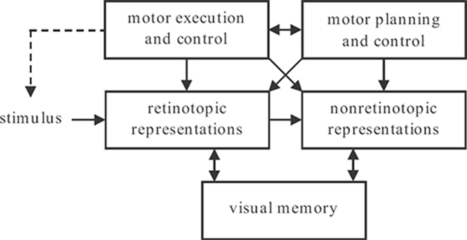
FIGURE 2.1
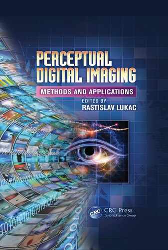
Schematic of the model. Visual inputs are first registered in retinotopic representations corresponding to early visual areas. A motion segmentation process transforms these into nonretinotopic representations. Visual memory is used to buffer information during the three-phase operation discussed in the next section. Motor systems include stages of motor planning and control that send command signals for motor execution and control, for example, for moving the eyes. Copies of efferent command and proprioceptive signals are available to modulate retinotopic and nonretinotopic representations. A motor action can either directly modify the stimulus, as in grasping, or shift the sensor (for example, the eye), thereby affecting the retinotopic stimulus indirectly. This relation between motor action and the stimulus is shown by a dashed arrow.
Using a similar stimulus, various studies investigated motion blur under conditions that include endogenous sources of blur [6], [7], [8], [9], [10], [11]. It was found that extra-retinal signals are used to reduce the spatial extent of motion blur.
Taken together, these results suggest that the human visual system uses stimulus-driven inhibitory interactions to limit the spatial extent of blur caused by exogenous sources. This strategy is augmented by use of extra-retinal signals to limit the spatial extent of blur caused by endogenous sources.
Figure 2.1 illustrates a schematic diagram of the model for how the visual system solves the problems of motion blur and moving ghosts. Visual inputs are first registered in retino-topic representations. Within retinotopic representations, moving targets generate extensively blurred (motion blur problem) and formless (moving ghosts problem) activities. The motion blur problem is addressed by retinotopic inhibitory interactions within retinotopic representations. In order to compute the form of moving objects, a motion grouping algorithm transforms retinotopic representations into nonretinotopic representations and stores them in visual short-term memory (VSTM). Endogenous sources of motion blur and moving ghosts problems are shown at the top of the figure. Motor control systems of the brain send efferent command signals to motor systems (control of eye, head, and body muscles) and a copy of these command signals is available for internal compensation. In addition, the vestibular system provides sensory signals about self-movement to initiate both motor and neural compensation. The details of where these internal (retinotopic and nonretinotopic) signals act to contribute to the solution of the motion blur and moving ghosts problems are not fully understood. Therefore, in Figure 2.1, these signals are represented as potentially available to both retinotopic and nonretinotopic representations.
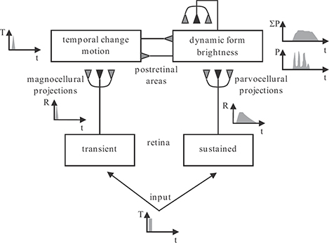
FIGURE 2.2
The RECOD model. The input is processed by retinal cells with transient and sustained response characteristics, giving rise to magnocellular and parvocellular pathways, respectively. The top layers show lumped representations of postretinal areas receiving their primary inputs from magnocellular and parvocellular pathways. Responses to a brief pulse input are shown in different parts of the model. Dark-gray and light-gray synaptic symbols indicate excitatory and inhibitory connections, respectively.
The rest of this chapter focuses on a computational model of how the spatial extent of motion blur can be controlled by stimulus-driven inhibitory interactions. For the nonretino-topic components of the general model shown in Figure 2.1, the reader is referred to recent reviews in References [12] and [13].
2.6 Retino-Cortical Dynamics Model
2.6.1 General Architecture
Figure 2.2 shows the schematic of the retino-cortical dynamics (RECOD) model [14]. The input is first processed by two populations of retinal ganglion cells, those with sustained and those with transient responses. The outputs of these two populations form two segregated pathways as they project from retina to visual cortex. These pathways are known as parvocellular and magnocellular pathways. In the visual cortex, one can distinguish neurons with sustained and those with transient responses. These populations are referred to as sustained and transient channels and correspond, mainly, to the cortical ventral and dorsal pathways. The ventral pathway is the main cortical system for processing figural properties, such as boundaries, surface features, color, etc. The dorsal pathway is the main cortical system for processing dynamic properties of stimuli, such as motion. Unlike pre-cortical areas, where parallel pathways remain segregated, in the cortex interactions exist between these two populations. These interactions can be both excitatory and inhibitory. The presented model emphasizes inhibitory interactions that play a critical role in motion deblurring. Thus, reciprocal inhibitory connections are shown between sustained and transient cortical channels. Since the problem of motion blur consists of smear in figural representations, the extent of smear in sustained pathways for moving targets is analyzed. It is also known that extensive feedback, including widespread positive feedback, exists in cortical areas. Because positive feedback can be a major source of hysteresis, and thus blur, these feedback connections are included in the analysis presented below.
FIGURE 2.3
Schematic illustration of the three-phase operation of the RECOD model. The top trace shows a step input that generates a short latency transient (M) and a longer latency sustained (P) response. The sustained response initially peaks to a value and decays thereafter to a lower plateau. The transient activity inhibits via transient-on-sustained inhibition the ongoing activity (shown in black) in postretinal sustained areas. This is the reset phase. Following this reset, the initial rise to a peak activity in the P response transfers the new input information to postretinal sustained areas and also activates feedback loops. This is the feedforward dominant phase. As the feedforward sustained activity decays to a lower plateau, the feedback activities overtake postretinal sustained responses. This is the feedback-dominant phase.
The operation of the model dynamics is summarized in Algorithm 2.1. The following discusses the original motivations for proposing the three-phase operation of the model.
Algorithm 2.1 The operation of the model dynamics.
Through the afferent retino-geniculate pathways, the onset of a stimulus evokes a fast transient magnocellular (M) activity and a slower sustained parvocellular (P) activity. These activities are shown schematically in Figure 2.3. The sustained response consists of an initial peak followed by a decay to a lower plateau value.
P and M activities flow predominantly to the dorsal and the ventral streams of cortical processing to initiate form/brightness and temporal-change/motion computations, respectively. Other P and M inputs to the dorsal and ventral pathways also exist to implement other functions and interactions between form and motion systems. Specifically, the model postulates reciprocal connections conveying M (P) input to the ventral (dorsal) pathway to implement reciprocal inhibition between these two pathways.
The temporal dynamics of the model in response to stimulus onset consists of three phases: reset phase, feedforward dominant phase, and feedback dominant phase.
At the stimulus onset, the fast transient activity inhibits via transient-on-sustained inhibitory connections any pre-existing activity at the retinotopic location of the new stimulus. This prevents the temporal integration and blurring of activities generated by different stimuli presented in temporal succession. This phase of operation is called the reset phase, because it is “resetting” the retinotopic locus of the new activity by removing any pre-existing activity.
As the sustained activity reaches its cortical locus, the initial peak of this activity transfers information from retina to cortex in a feedforward manner. This phase of operation is called the feedforward-dominant phase, because signals in the feedforward connections dominate signals in the feedback connections.
As the feedforward signals become registered in cortical areas, they activate feedback loops. The decay of the afferent sustained activity to a lower plateau level allows feedback signals to dominate in cortex, giving rise to feedback dominant phase of operation.
When a change occurs in the input signal, the whole cycle repeats itself.
Form synthesis under natural viewing conditions is an extremely difficult problem. The appearance of the stimuli and the context can change drastically within and across scenes. Feedforward architectures do not have the flexibility required to handle these complex problems. As a result, feedback, both positive and negative, is required for processing natural visual stimuli. In fact, the visual cortex contains massive feedback connections. However, a major problem with positive feedback is that it can drive the system toward unstable behavior. To address this problem, it has been suggested that the visual system is designed to operate in a succession of transient regimes to avoid uncontrolled explosion of activity that would result from a sustained positive feedback signaling. When an input changes, a fast transient activity is used to reset the ongoing activity. In the feedforward-dominant phase, input signals are conveyed to cortical areas with the strong initial overshoot of the activity in the sustained pathway. This allows fast registration of new inputs. After this initial registration, the feedforward signal decays to a lower plateau, where the signal is strong enough to maintain a cortical activity but not too strong to override figural synthesis by feedback signaling. Thus, the third phase consists of feedback-dominant operation, where feedback signals carry out figural synthesis. Overall, these phases last a few hundred milliseconds. The next reset can occur either exogenously by changes in the stimulus, which generate reset signals in the retinotopic map at the location of the change, or endogenously by self-generated motion, which in turn causes global changes and thus a global reset in the retinotopic map. As discussed in the next subsection, this three-phase operation provides a natural explanation to how the visual system deals with the motion blur problem.
2.6.2 Mathematical Description
The model is based on general types of differential equations used to describe the behavior of neurons, populations of neurons, and the behavior of biochemical dynamics. The first type of equation used in the model has the form of a generic Hodgkin-Huxley equation
where Vm represents the membrane potential, gp, gd, and gh are the conductances for passive, depolarizing, and hyperpolarizing channels, respectively, with Ep, Ed, and Eh representing their Nernst potentials.
The above equation has been used extensively in neural modeling to characterize the dynamics of membrane patches, single cells, as well as networks of cells [15]. To put the model in an equivalent but simpler form, let Ep = 0 and use the symbols B, D, and A for Ed, Eh, and gp, respectively, to obtain the generic form for multiplicative or shunting equation [15]:
The depolarizing and hyperpolarizing conductances are used to represent the excitatory and inhibitory inputs, respectively. The second type of equation, called the additive, leaky-integrator model,
is a simplified version of Equation 2.2. The influence of external inputs on membrane potential occurs directly as depolarizing (Id) and hyperpolarizing (Ih) currents, instead of conductance changes.
Shunting networks can automatically adjust their dynamic range, allowing them to process small and large inputs [15]. Accordingly, shunting equations can be used in the case of interactions among a large number of neurons so that a given neuron can maintain its sensitivity to a small subset of its inputs without running into saturation when a large number of inputs become active. The proposed model uses the simplified additive equations when the interactions involve few neurons.
Finally, a third type of equation is used to express biochemical reactions of the form
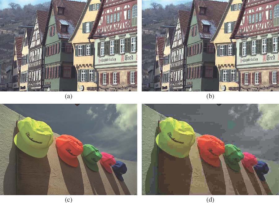
FIGURE 3.3
The effect of the contrast masking property of human vision on visual quality using JPEG compression: (a) original Building image, (b) its distorted version with MSE = 134.61, (c) original Caps image, and (d) its distorted version with MSE = 129.24. The distorted images clearly differ in their visual quality, although they have similar MSE with respect to the original.
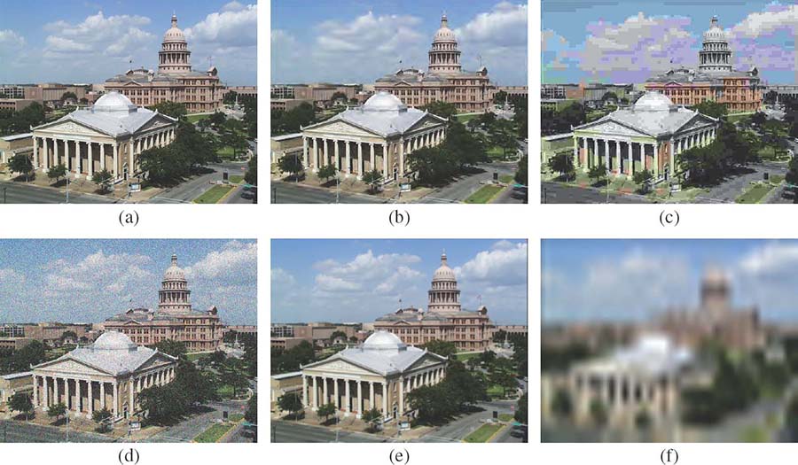
FIGURE 3.4
Example distortions from the LIVE IQA database: (a) original image, (b) JPEG2000 compression, (c) JPEG compression, (d) white noise, (e) blur, and (f) Rayleigh fading.
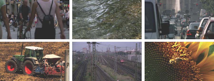
FIGURE 3.5
Sample frames from the LIVE VQA database.

FIGURE 4.1
Images with different aesthetic qualities. Images on the first row are taken by professional photographers while images on the second row are taken by amateur photographers.
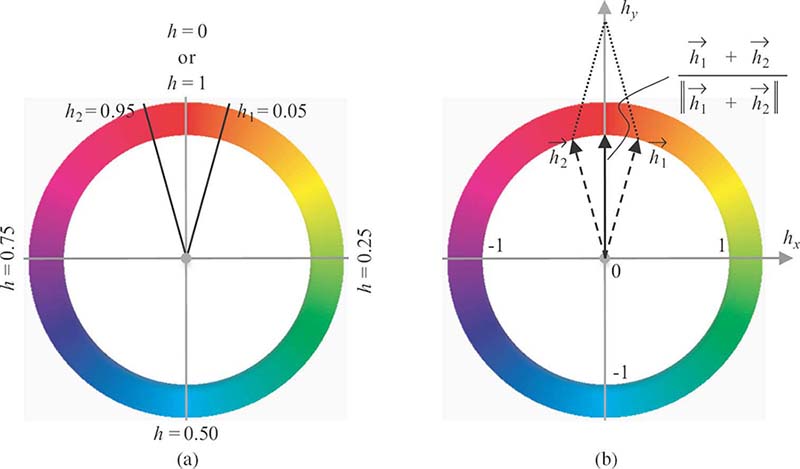
FIGURE 4.4
Different representations of the hue values: (a) scalar representation and (b) vector representation.
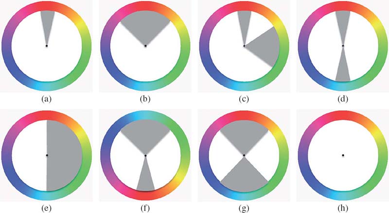
FIGURE 4.5
Harmony hue distribution models with gray indicating the efficient regions: (a) i type, (b) V type, (c) L type, (d) I type, (e) T type, (f) Y type, (g) X type, and (h) N type. All the models can be rotated by an arbitrary angle.
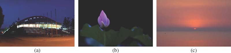
FIGURE 4.6
Image examples that fit with different types of hue harmony models in Figure 4.5: (a) fitting I-type harmony, (b) fitting Y-type harmony, and (c) fitting i-type harmony.
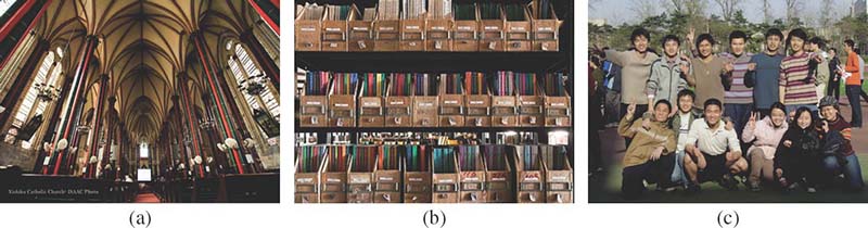
FIGURE 4.9
Texture and patterns. Patterns in these examples evoke aesthetic feelings.
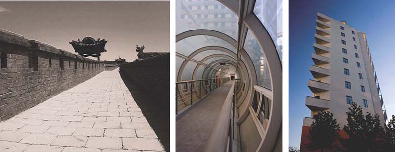
FIGURE 4.10
Linear perspective in photographs.

FIGURE 5.5
An illustration of exposure: (a) portrait with a dark background and perceptual exposure, (b) portrait with a light background and perceptual exposure, (c) portrait with a dark background and naive mean value exposure, and (d) portrait with a light background and naive mean value exposure.
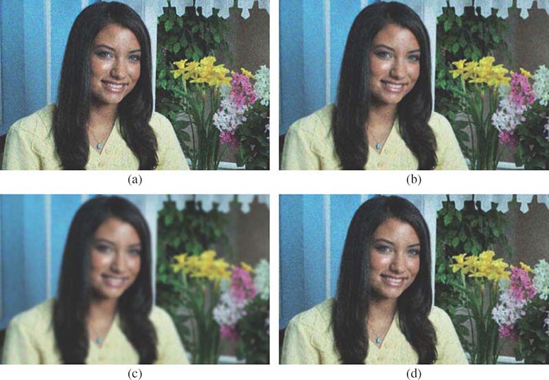
FIGURE 5.14
Example images with: (a) noise, (b) light RGB smoothing, (c) aggressive RGB smoothing, and (d) simple color opponent smoothing.
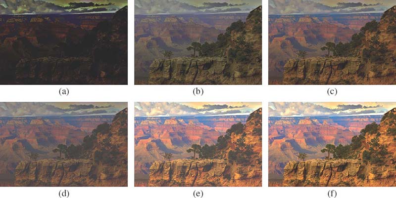
FIGURE 5.15
A series of images illustrating how an image approximately appears when displayed on a monitor at different steps in the color rendering, where (a–c) simulate images viewed within a flareless viewing environment and images (d–f) simulate images viewed with flare. (a) The original linear camera image, (b) after gamma correction but not color corrected, (c) after color correction and gamma correction, (d) after color correction and gamma correction (with flare), (e) with boosted RGB scales, and (f) after flare correction.
FIGURE 5.18
Example images with: (a) no edge enhancement, (b) linear edge enhancement, and (c) soft thresholding and edge-limited enhancement.

FIGURE 6.1
The Macbeth color checker taken under the (a) daylight, (b) tungsten, and (c) fluorescent illumination.
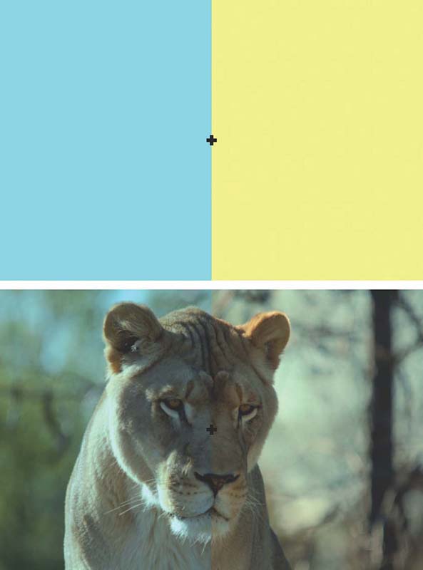
FIGURE 6.3
Chromatic adaptation. Stare for twenty seconds at the cross in the center of the top picture. Then focus on the cross in the bottom picture; the color casts should disappear and the image should look normal.
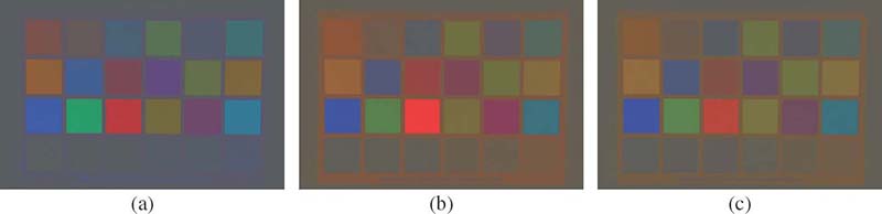
FIGURE 6.8
Chrominance representation of the images shown in Figure 6.1 for the (a) daylight, (b) tungsten, and (c) fluorescent illumination.
FIGURE 6.9
Examples of the images taken in different lighting conditions without applying white balancing.

FIGURE 6.10
Joint white balancing and color enhancement using the spectral modeling approach: (a,d) r = 0, (b,e) r = 0.25, and (c,f) r = 1.0.
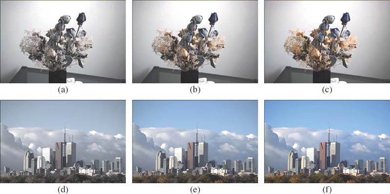
FIGURE 6.11
Joint white balancing and color enhancement using the spectral modeling approach: (a,d) r = − 0.5, (b,e) r = 0, and (c,f) r = 0.5.
FIGURE 6.12
Joint white balancing and color enhancement using the combinatorial approach: (a,d) w = 0.5, (b,e) w = 0, and (c,f) w = − 0.5.
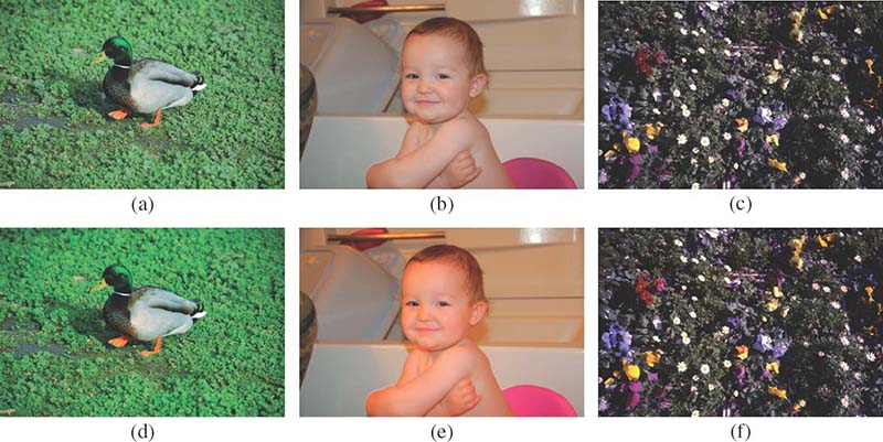
FIGURE 6.13
Color enhancement of images with inaccurate white balancing: (a–c) input images and (d–f) their enhanced versions.

FIGURE 6.14
Color adjustment of the final camera images: (a,d) suppressed coloration, (b,e) original coloration, and (c,f) enhanced coloration.
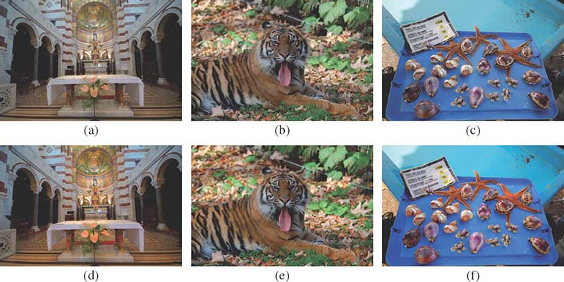
FIGURE 6.15
Color enhancement of the final camera images: (a–c) output camera images and (d–f) their enhanced versions.
FIGURE 7.1
Signal-level thumbnail generation: (a) original image, (b) two magnified regions cropped from the original image, and (c–f) thumbnails. Thumbnails are downsampled using (c) decimation, (d) bilinear, (e) bicubic, and (f) Lanczos filtering.
FIGURE 7.2
ROI-based thumbnail generation: (a) high-resolution image, (b) automatic cropping, and (c) seam carving.
FIGURE 7.3
Quality-indicative visual cues: (a) blur, (b) noise, (c) bloom, and (d) red-eye defects.

FIGURE 7.12
Highlighting blur in the thumbnail when the original image is blurred: (a) conventional thumbnail at a resolution of 423 × 317 pixels, (b) two magnified regions from the original image with 2816 × 2112 pixels, (c) perceptual thumbnail obtained using gradient-based blur estimation, (d) corresponding blur map, (e) perceptual thumbnail obtained using the scale-space-based blur estimation, and (f) corresponding blur map.
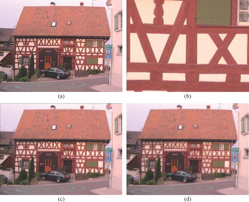
FIGURE 7.13
Highlighting blur in the thumbnail when the original image is sharp: (a) conventional thumbnail with 341 × 256 pixels, (b) magnified region from the original image with 2048 × 1536 pixels, (c) perceptual thumbnail via gradient-based blur estimation, and (d) perceptual thumbnail via scale-space-based blur estimation.

FIGURE 7.14
Highlighting blur in the thumbnail when the original image with 1536 × 2048 pixels is sharp: (a) conventional thumbnail with 256 × 341 pixels, (b) perceptual thumbnail via gradient-based blur estimation, and (c) perceptual thumbnail via scale-space-based blur estimation.
FIGURE 7.18
Highlighting blur and noise in the thumbnail: (a) original image with both blur and noise, (b) two magnified regions from the original image, (c) conventional thumbnails obtained using bilinear filtering, (d) conventional thumbnails obtained using bicubic filtering, (e) conventional thumbnails obtained using Lanczos filtering, (f) gradient-based estimation blur map, (g) perceptual thumbnail obtained using gradient-based blur estimation, (h) perceptual thumbnail obtained using gradient-based blur estimation and region-based noise estimation, (i) scale-space-based estimation blur map, (i) perceptual thumbnail obtained using scale-space-based blur estimation, and (k) perceptual thumbnail obtained using scale-space-based blur estimation and multirate noise estimation.
FIGURE 11.2
Top six ranks of correlogram retrieval in two image databases with (a) 10000 images and (b) 20000 images. Top-left is the query image.

FIGURE 11.5
Four queries in Corel 10K database: (a–d) correlogram for d = 10, (e–h) perceptual correlogram for d = 10, and (i–l) perceptual correlogram for d = 40. Top-left is the query image.
FIGURE 11.6
Retrieval result of the perceptual correlogram for the query in Figure 11.2.
FIGURE 11.7
A special case where the correlogram works better than the perceptual correlogram descriptor: (a) correlogram and (b) perceptual correlogram.
FIGURE 11.15
Four typical queries using three descriptors in Corel 10K database: (a–d) dominant color, (e–h) correlogram, and (i–l) proposed method. Top-left is the query image.

FIGURE 11.16
Four typical queries using three descriptors in Corel 20K database: (a–d) dominant color, (e–h) auto-correlogram, and (i–l) proposed method. Top-left is the query image.

FIGURE 11.17
Two queries in (a,b,e,f) Corel 10K and (c,d,g,h) Corel 20K databases where (auto-)correlogram performs better than SCD: (a,e) correlogram, (b,f) proposed method, (c,g) auto-correlogram, and (d,h) proposed method. Top-left is the query image.

FIGURE 12.1
An input image and its coarse segmentation.
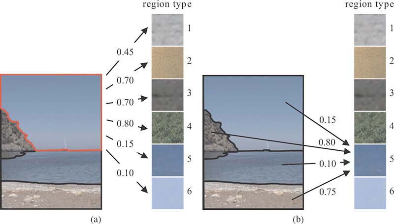
FIGURE 12.4
Distances between regions and region types: (a) distances between an image region and all region types; (b) distances between all regions and a specific region type.
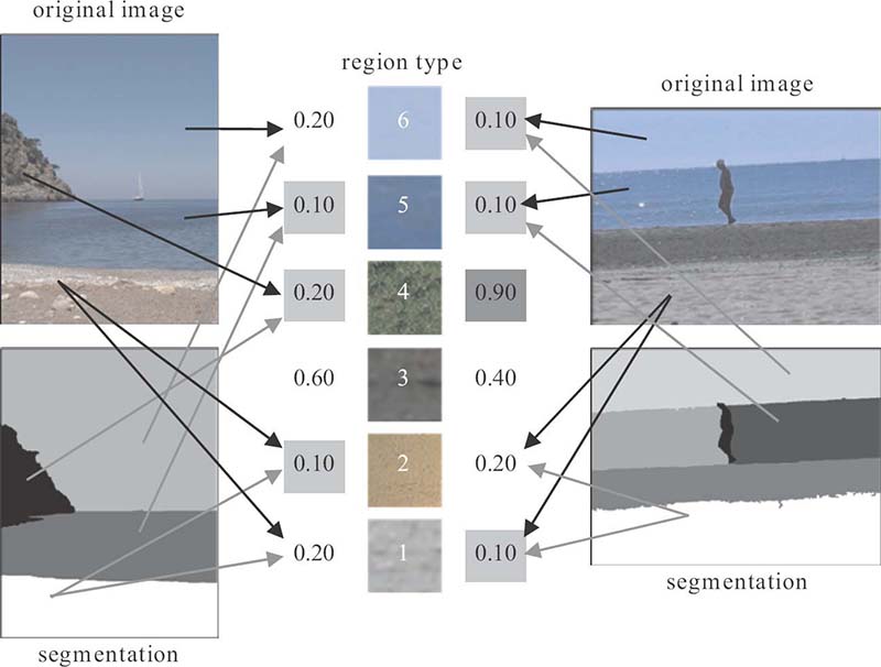
FIGURE 12.5
Construction of model vectors for two images and a visual thesaurus of six region types; lowest values of model vectors are highlighted (light gray) to note which region types of the thesaurus are most contained in each image, whereas a high value (dark gray) indicates a high distance between the corresponding region type and the image.
FIGURE 12.10
An example from the Beach domain, where the region types of an image are different than a typical Beach image.
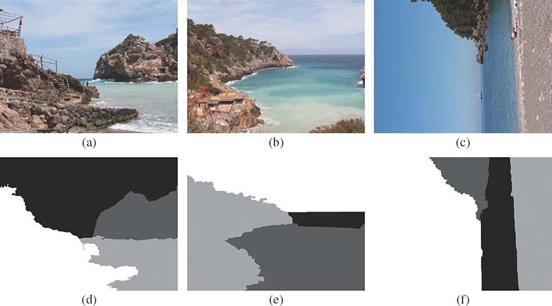
FIGURE 12.15
Three examples from the Beach domain. Initial images and their segmentation maps.

FIGURE 12.16
Indicative Corel images.
FIGURE 12.17
Indicative TRECVID images.
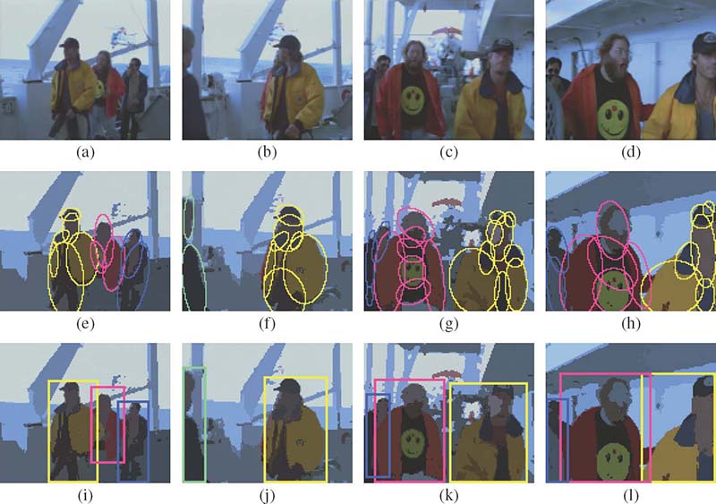
FIGURE 13.4
PGA performance demonstration on a sequence from Titanic movie: (a,e,i) frame 77, (b,f,j) frame 103, (c,g,k) frame 142, and (d,h,l) frame 175. (a–d) Original frames, (e–h) PGA-identified foreground blobs on the DSCT color-clustered frame, and (i–l) perceptual clusters marked with the same color as the blobs belonging to the distinct foreground clusters. Note that the person wearing the red jacket, initially seen on the right of the person wearing the yellow jacket, comes to the left starting from frame 110.
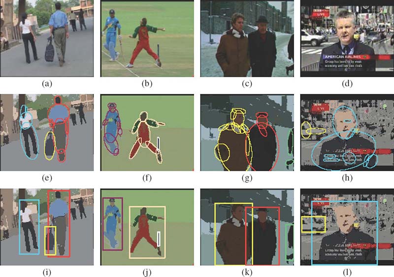
FIGURE 13.5
PGA performance demonstration on various scenes: (a–d) original frames in four different scenes, (e–h) identified foreground blobs, and (i–l) perceptual clusters.
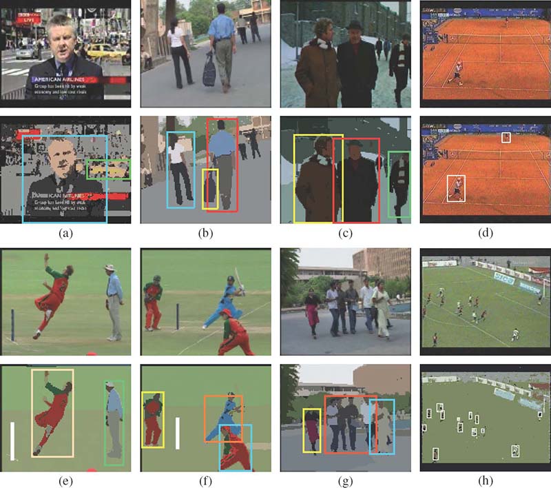
FIGURE 13.8
Scene categorization: (a–d) subject-centric scenes, as they all have one or two prominent subjects, which exist throughout the duration of the shot, and (e–h) frame-centric scenes because the subjects in these scenes last only for a small duration in the shot. Prominence values for the subjects taken from left to right: (a) {0.96,0.1}, (b) {0.3, 0.8, 0.95}, (c) {0.8, 0.8, 0.18}, (d) {0.61, 0.66}, and (e–h) values smaller than 0.5 according to the proposed prominence model which includes life span as an attribute.
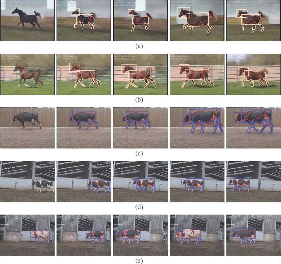
FIGURE 13.11
Results obtained for various horse and cow videos. Probability at node E: (a) 0.814, (b) 0.795, (c) 0.910, (d) 0.935, and (e) 0.771, 0.876, 0.876, 0.800, and 0.911 for different videos with the object model cow.
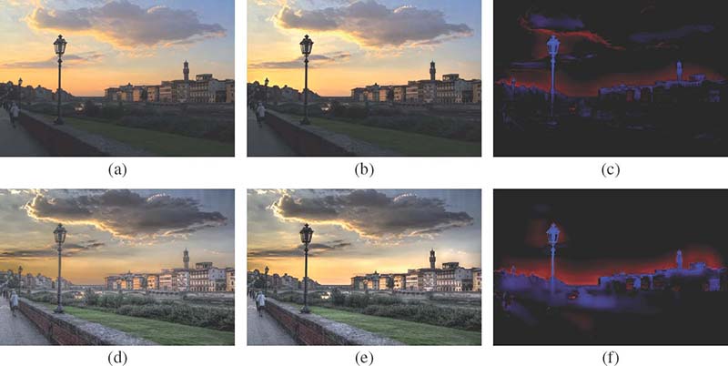
FIGURE 15.3
Two examples of how the Cornsweet illusion can enhance the contrast of tone-mapped images are presented on the left. (a–c) Example processed using a global tone mapping operator, where countershading restores contrast in the heavily compressed dynamic range of the sky and highlights. (d–f) Example processed using a local tone mapping operator, which emphasizes on local details at expense of losing global contrast between the landscape and sky. In this case countershading restores brightness relations in this starkly detailed tone mapping result. Notice that the contrast restoration preserves the particular style of each tone mapping algorithm.
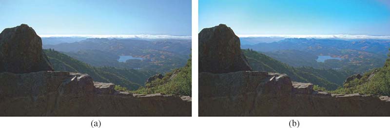
FIGURE 15.4
The Cornsweet illusion used for color contrast enhancement: (a) original image and (b) its enhanced version using Cornsweet profiles in the chroma channel. In this example, the higher chroma contrast improves the sky and landscape separation and enhances the impression of scene depth.

FIGURE 15.9
The glare appearance example [22]. ©The Eurographics Association 2009
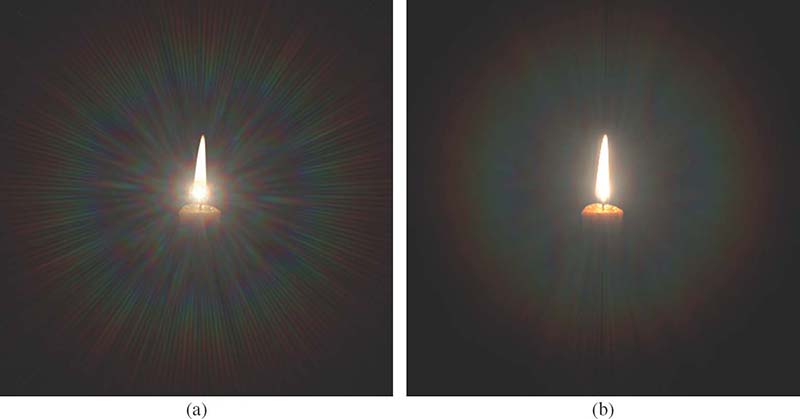
FIGURE 15.12
The glare appearance for a luminous object of non-negligible spatial size [22]: (a) the light diffraction pattern (point-spread function) is just imposed on the background candle image, (b) the light diffraction pattern is convolved with the image. ©The Eurographics Association 2009.
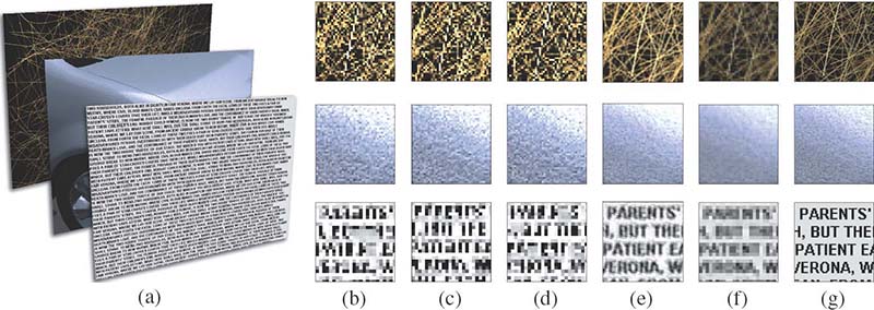
FIGURE 15.17
Resolution enhancement: (a) test images, (b–d) subimages obtained in the optimization process, (e) resolution enhancement via simulation of the images created on the retina once the three subimages are shown on a high frame rate display, (f) Lanczos downsampling as a standard method, and (g) original high-resolution images. Note, that even though the resolution was reduced three times, the presented method was able to recover fine details in contrast to the standard downsampling method.
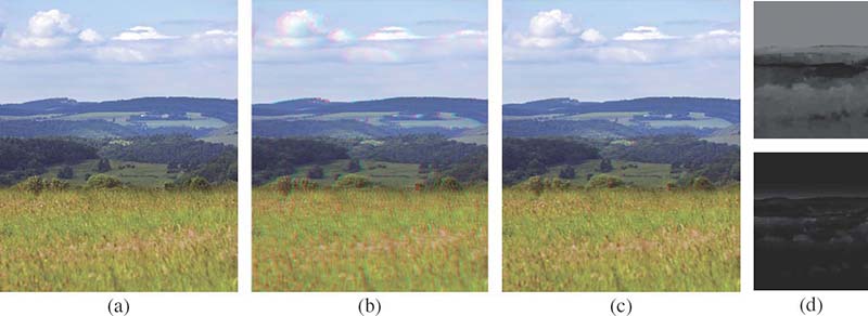
FIGURE 15.20
Backward-compatible anaglyph stereo (c) offers good depth-quality reproduction with similar appearance to the standard stereo image. The small amount of disparity leads to relatively high-quality images when stereo glasses are not used. To achieve equivalent depth-quality reproduction in the traditional approach significantly more disparity is needed (b), in which case the appearance of anaglyph stereo image is significantly degraded once seen without special equipment.
FIGURE 15.21
Depth enhancement using the Cornsweet illusion for two different scenes with significant depth range: (a,c) original images and (b,d) enhanced anaglyph images. A better separation between foreground and background objects and a more detailed surface structure depiction can be perceived in enhanced images.
where a biochemical agent S, activated by the input, interacts with a transducing agent Z (e.g., a neurotransmitter) to produce an active complex Y that carries the signal to the next processing stage. This active complex decays to an inactive state X, which in turn dissociates back into S and Z. It can be shown (see Appendix in Reference [16]) that when the active state X decays very fast, the dynamics of this system can be written as follows:
with the output given by , where S(t), z(t), and y(t) represent the concentrations of S, Z, and Y, respectively. Parameters γ, δ, and α denote rates of complex formation, decay to inactive state, and dissociation, respectively. The parameter t dictates the overall speed of the reaction. This equation has been used in a variety of neural models, in particular to represent temporal adaptation, or gain control property, occurring for example through synaptic depression.
These fundamental equations can be now used to develop model equations. The retino-topic representation is a spatially two-dimensional representation. For simplicity, a one-dimensional model is built, and an index for each variable is used to denote its location in the retinotopic representation.
The first step in retinal processing is temporal adaptation realized by using Equation 2.5 as follows:
where zi represents the concentration of a transducing agent, such as a neurotransmitter, for a neuron positioned at the ith retinotopic location, J is a baseline signal determining baseline concentration, and Ii is the external input (luminance) impinging on the ith retinotopic location. This transducing stage provides input to a retinal network that generates the output of the sustained, or parvocellular, cells. These cells have concentric center-surround receptive field organization and are described by the shunting equation (Equation 2.2) adapted as follows:
The conductance values gd and gh controlling the depolarization and hyperpolarization of the membrane potential in Equation 2.2 have been replaced by depolarizing and hyper-polarizing terms that consist of the sum of baseline signal Js and external input Ij at the jth retinotopic location multiplied by the concentration of the transducing agent zj. These inputs are then weighted by Gaussian functions and of retinotopic distance j − i. The superscript s denotes that the baseline input and the Gaussian function is for sustained cells. The superscripts e and i indicate that the Gaussian function relates to the excitatory and inhibitory components, respectively, of the difference of Gaussian receptive field profile of sustained cells. The parameter ns determines the spatial extent of the Gaussian in the retinotopic space. The output of each sustained cell is fed to an additive equation
where the parameter σ determines the decay rate of the activity, λ is a constant representing the gain the the transformation of membrane potential to spike rate and [.]+ is the half-wave rectification function with parameter γs representing the spiking threshold of the neuron. These equations together generate the sustained response profile shown in Figure 2.3, where a step input generates a peak that decays to a lower plateau due to the adaptation dynamics described by Equation 2.6.
Retinal cells with transient activities (magnocellular) obey a similar but simpler equation
Here the substraction of the delayed version of the input (delay is equal to δ) implements a backward differentiation scheme and generates transient responses as shown schematically in Figures 2.2 and 2.3.
The postretinal network provides a lumped representation of visual areas beyond the retina (LGN and visual cortical areas). Here again, cells with sustained and transient activities are represented as those found in various visual cortical areas. However, unlike the retina where sustained and transient systems are isolated from each other, direct interactions between them are introduced here. In fact, it is known that parvo (sustained) and magno (transient) pathways remain separate until they reach visual cortex and constitute the main inputs to ventral and dorsal cortical streams. On the other hand, a variety of evidence shows that there exists a certain level intermixing between the pathways at the cortical level supporting the view of reciprocal interactions. While, both excitatory and inhibitory interactions can occur between these two systems, the focus here is on reciprocal inhibitory interactions, which are critical in explaining the motion deblurring phenomenon.
Accordingly, postretinal cells mainly driven by the parvocellular (sustained) pathway are described by the shunting equation
The excitatory term contains positive feedback Φ(pi) and the afferent signal from the sustained parvocellular pathway vi, which is subject to delay η. The inhibitory term consists of inhibitory feedback Φ(pj), inhibitory surround component of the afferent sustained signal vj, and the inhibition from transient postretinal cells mj. Terms and are Gaussian weights of the inhibitory signals used to shape the receptive field.
Postretinal inhibitory interneurons carry inhibition from postretinal sustained cells to postretinal transient cells. They are described by the additive equation
where qi is the activity of the ith postretinal interneuron.
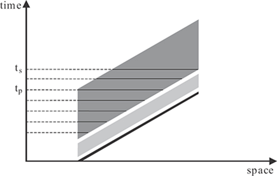
FIGURE 2.4
Space-time diagram depicting activities in the RECOD model for a single dot moving to the right with a constant speed. The black line represents the stimulus and the light-gray and dark-gray areas represent the transient and sustained responses, respectively. The length of horizontal lines across the sustained activity at different time instants indicate the spatial extent of motion blur for corresponding exposure durations. The spatial extent of motion blur increases linearly until the tp and remains constant until the time corresponding to the last visible point of the stimulus (ts).
Finally, the equation for postretinal neurons mainly driven by magnocellular pathway is given by
where mi is the activity of the ith postretinal transient cell and the function [.]++ denotes full wave rectification generating on-off response characteristics of these transient cells. The parameter κm is the relative delay of the intrachannel inhibition with respect to the excitatory signal.
2.7 Motion Deblurring
In order to understand why an isolated target generates motion blur but a dense array of targets do not, consider the following simplified scenario. Assume one-dimensional space and, as an isolated target, consider a single dot moving with a constant speed. The activities that would be generated by the model for such a stimulus are depicted in the space-time diagram of Figure 2.4. A dot moving at a constant speed corresponds to an oriented line in the space-time diagram. In response to this stimulus, a fast-transient and a slower-sustained activity are generated. The sustained activity decays slowly and, as a result, persists for a considerable time period (for example, 150 ms). As shown by the horizontal lines at various time instants in the figure, the spatial extent of motion blur increases as a function of exposure duration until it reaches a plateau at an exposure duration equal to the duration of visible persistence (tp). The spatial extent of blur can be converted to an equivalent duration of blur by dividing it by the speed of the stimulus. If the duration of blur is plotted as a function of exposure duration, one would find a linear increase for the duration of blur with a slope of one until it reaches the critical value of the duration of visible persistence. After this value, it remains constant. This explains why an isolated target appears blurred and why the extent of spatial blur increases with exposure duration.
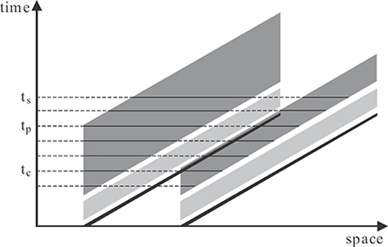
FIGURE 2.5
Space-time diagram depicting activities in the RECOD model for two dots moving to the right with a constant speed. The black lines represent the stimuli and the light-gray and dark-gray areas represent the transient and sustained responses, respectively. The length of horizontal lines across the sustained activity at different time instants indicate the spatial extent of motion blur for corresponding exposure durations. For the trailing dot, the spatial extent of motion blur increases linearly with exposure duration. The spatial extent of motion blur for the leading dot increases linearly like the trailing dot until tc when the transient activity of the trailing dot starts inhibiting the sustained activity of the leading dot.
To understand why an array of dots does not appear blurred, consider the simple scenario where two dots travel at the same speed as shown in Figure 2.5. For the trailing dot, one obtains the same result as a single dot. However, as one can see from the figure, there will be a spatiotemporal overlap between the sustained activity of the leading dot and the transient activity of the trailing dot. According to the RECOD model, the transient-on-sustained inhibition (term in Equation 2.10) will inhibit the sustained activity of the leading dot, thereby reducing the spatial extent of motion blur. If the duration of blur is plotted as a function of exposure duration, one can see that, initially, the duration of blur increases the same way for the leading and the trailing dots until the critical time tc, where the transient activity of the trailing dot starts inhibiting the sustained activity of the leading dot. After tc, the duration of motion blur for the leading dot remains constant, while the duration of blur for the trailing dot continues to increase.
These simple predictions of the RECOD model were tested by psychophysical experiments [5]. The results are shown in Figure 2.6. The left and right panels show data for the leading and trailing dots, respectively, for two spatial separation values between these two dots. For the trailing dot, the duration of blur increases linearly as a function of exposure duration with little effect of dot-to-dot separation. In contrast, for the trailing dot, the linear increase is curtailed beyond exposure duration of approximately 100 ms. Moreover, this motion deblurring is more prominent when the dot-to-dot separation is small. As it can be seen in Equation 2.10, transient-on-sustained inhibition is weighted by a retino-topic distance-dependent Gaussian function . Moreover, as the dynamics of differential equations in Section 2.6 suggests, the decay in the activity of the neurons is gradual. As a result, the effects depicted in Figures 2.4 and 2.5 occur in a more gradual way in the model compared to the schematic representations shown in these figures. In order to obtain quantitative predictions from the model and compare them to data, the model was simulated by using a numerical ordinary differential equation solver [17]. The results are plotted against the data in Figure 2.6. The good fit between model predictions and data provides support for the proposition that spatial extent of motion blur is controlled by inhibitory interactions between sustained and transient systems within retinotopic representations.
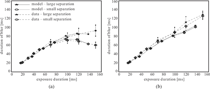
FIGURE 2.6
Motion deblurring data and model predictions for two dot-to-dot separations [17]: (a) the leading dot and (b) the trailing dot. ©1998 Elsevier
2.8 Conclusion
This chapter reviewed conditions that prevail under normal ecological vision by human observers. The sources of motion can be divided into exogenous and endogenous categories. The former refers to motion outside the observer; for example, when a car approaches the observer. The latter refers to motion resulting from the observer; for example, when the observer moves his/her head or eyes. This categorization is useful in that it allows to draw fundamental distinctions in resulting dynamic images. Namely, endogenous motion generates global retinotopic motion with a correlated retinotopic motion field, and it can be predicted and/or corrected by use of internal signals that control the motion of the observer. In contrast, exogenous motion is often localized in the visual field and lacks global correlation. Given these fundamental differences, it was suggested that the human nervous system uses a variety of strategies suited to each condition.
The second part of the chapter focused on the problem of motion blur and outlined a model of retino-cortical dynamics, called RECOD. It was shown that inhibitory interactions within retinotopic representations can reduce the spatial extent of motion blur. In this ongoing research, the complementary problem of moving ghosts is investigated. As shown in Figure 2.1, retinotopic representations are transformed into nonretinotopic representations — a fundamental factor in this transformation is the establishment of a new nonretinotopic reference frame. It was further suggested that motion grouping plays a critical role in establishing these reference frames. Gestalt psychologists noticed the tendency of stimuli sharing a common motion direction to group together and called this the grouping law of common faith. As mentioned above, for exogenous sources of motion, the resulting retinotopic patterns are local and necessitate a segmentation and a grouping process to identify and isolate each locus of common motion. Grouping by common faith can achieve this goal thereby leading to the transformation of retinotopic representations to nonretinotopic ones. Motion deblurring in retinotopic representations along with dynamic form computation in nonretinotopic representations can together explain how the visual system solves simultaneously the motion blur and moving ghosts problems.
Acknowledgment
Figure 2.6 is reprinted from Reference [17] with the permission from Elsevier.
References
[1] J. Gibson, “Ecological optics,” Vision Research, vol. 1, no. 3–4, pp. 253–262, October 1961.
[2] H. Collewijn and J. Smeets, “Early components of the human vestibulo-ocular response to head rotation: Latency and gain,” Journal of Neurophysiology, vol. 84, no. 1, pp. 376–389, July 2000.
[3] A. Charpentier, “Recherches sur la persistence des impressions retiniennes et sur les excitations lumineuses de courte duree,” Arch Ophthalmol, vol. 10, pp. 108–135, 1890.
[4] D. Burr, “Motion smear,” Nature, vol. 284, no. 5752, pp. 164–165, March 1980.
[5] S. Chen, H. Bedell, and H. Ogmen, “A target in real motion appears blurred in the absence of other proximal moving targets,” Vision Research, vol. 35, no. 16, pp. 2315–2328, August 1995.
[6] H.E. Bedell, J. Tong, and M. Aydin, “The perception of motion smear during eye and head movements,” Vision Research, vol. 50, no. 24, pp. 2692–2701, December 2010.
[7] J. Tong, S.B. Stevenson, and H.E. Bedell, “Signals of eye-muscle proprioception modulate perceived motion smear,” Journal of Vision, vol. 8, no. 14, pp. 7.1–6, October 2008.
[8] J. Tong, M. Aydin, and H.E. Bedell, “Direction and extent of perceived motion smear during pursuit eye movement,” Vision Research, vol. 47, no. 7, pp. 1011–1019, March 2007.
[9] J. Tong, S. Patel, and H. Bedell, “The attenuation of perceived motion smear during combined eye and head movements,” Vision Research, vol. 46, no. 26, pp. 4387–4397, December 2006.
[10] H. Bedell and S. Patel, “Attenuation of perceived motion smear during the vestibulo-ocular reflex,” Vision Research, vol. 45, no. 16, pp. 2191–2200, July 2005.
[11] H. Bedell, S. Chung, and S. Patel, “Attenuation of perceived motion smear during vergence and pursuit tracking,” Vision Research, vol. 44, no. 9, pp. 895–902, April 2004.
[12] H. Ogmen, “A theory of moving form perception: Synergy between masking, perceptual grouping, and motion computation in retinotopic and non-retinotopic representations,” Advances in Cognitive Psychology, vol. 3, no. 1–2, pp. 67–84, July 2007.
[13] H. Ogmen and M.H. Herzog, “The geometry of visual perception: Retinotopic and nonretino-topic representations in the human visual system,” Proceedings of the IEEE, vol. 98, no. 3, pp. 479–492, March 2010.
[14] H. Ogmen, “A neural theory of retino-cortical dynamics,” Neural Networks, vol. 6, no. 2, pp. 245–273, 1993.
[15] S. Grossberg, “Nonlinear neural networks – Principles, mechanisms, and architectures,” Neural Networks, vol. 1, no. 1, pp. 17–61, 1988.
[16] M. Sarikaya, W. Wang, and H. Ogmen, “Neural network model of on-off units in the fly visual system: Simulations of dynamic behavior,” Biological Cybernetics, vol. 78, no. 5, pp. 399– 412, May 1998.
[17] G. Purushothaman, H. Ogmen, S. Chen, and H. Bedell, “Motion deblurring in a neural network model of retino-cortical dynamics,” Vision Research, vol. 38, no. 12, pp. 1827–1842, June 1998.