
9
Perceptually Driven Super-Resolution Techniques
Nabil Sadaka and Lina Karam
9.2 Main Super-Resolution Techniques
9.2.1 Single-Frame Super-Resolution
9.2.2 Multi-Frame Super-Resolution
9.3 Multi-Frame Super-Resolution Observation Model
9.4 Super-Resolution Problem Formulation
9.4.1 Bayesian Super-Resolution Formulation
9.4.2 Regularized-Norm Minimization Formulation
9.4.3 Non-Iterative Kernel-Based Formulation
9.4.4 Super-Resolution Solutions in Practice
9.5 Perceptually Driven Efficient Super-Resolution
9.5.1 Selective Perceptual Super-Resolution Framework
9.5.2 Perceptual Contrast Sensitivity Threshold Model
9.5.3 Perceptually Significant Pixels Detection
9.6 Attentively Driven Efficient Super-Resolution
9.6.1 Attentive-Selective Perceptual Super-Resolution Framework
9.6.2 Saliency-Based Mask Detection
9.6.2.1 Hierarchical Saliency Model
9.6.2.2 Foveated Saliency Model
9.6.2.3 Frequency-Tuned Saliency Model
9.7 Perceptual SR Estimation Applications
9.7.1 Perceptual MAP-Based SR Estimation
9.7.2 Perceptual Fusion-Restoration SR Estimation
9.7.3 Perceptually Driven SR Results
9.1 Introduction
Nowadays, high-resolution (HR) image/video applications are reaching every home and soon will become a necessity rather than a mere luxury. Whether it is through a high-definition (HD) television, computer monitor, HD camera, or even a handheld phone, HR multimedia applications are becoming essential components of consumers’ daily lives. Moreover, the demand for HR images transcends the need for offering a better-quality picture to the common viewer. HR imagery is continuing to gain popularity and dominate many industries that require accurate image analysis. For example, in surveillance applications, high-resolution images are needed for a better performance of target detection, face recognition, and text recognition [1], [2]. Furthermore, medical imaging applications require HR images for accurate assessment and detection of small lesions [3], [4].
The capture and delivery of HR multimedia content is a complex and problematic process [5]. In any typical imaging system or multimedia delivery chain, the quality of HR media can be impaired by processes of acquisition, transmission, and display. The resolution of the imaging systems is physically limited by the pixel density in image sensors. On one hand, increasing the number of pixels in an image sensor via reducing the pixel size is limited by the existence of shot noise and associated high cost. On the other hand, increasing the chip size is deemed ineffective due to the existence of a large capacitance that slows the charge transfer rate and limits the data transfer [6]. Thus, a major drawback of HR image acquisition in many of the aforementioned applications is the inadequate resolution of the sensors, either because of cost or hardware limitation [7]. In addition to hardware limitations, HR imagery can be blurred during acquisition due to atmospheric turbulence and the camera-to-object motion [8]. Transmission of HR media requires extremely high bandwidth, which is usually not available in real-time scenarios. Thus, high compression rates are imposed on the media content, resulting in annoying compression artifacts and high frame dropping rates [9]. Moreover, large displays use interpolation techniques to scale video content to fit a target screen size, thus introducing blurred details and system noise enlargement. Hence, advanced signal processing, such as super-resolution (SR) imaging, offers a cost-effective way to increase image resolution by overcoming sensor hardware limitations and reducing media impairments.
When choosing a solution for the SR problem, there is always a trade-off between computational efficiency and HR image quality. Existing SR approaches suffer from extremely high computational requirements due to the high dimensionality in terms of large number of unknowns to be estimated when solving the SR inverse problem. Recently, SR techniques are at the heart of HR image/video technologies in various application areas, such as consumer electronics, entertainment, digital communications, military, and biomedical imaging. Most of these applications require real-time or near real-time processing due to limitations on computational power with the essential demand for high image quality requirements. Efficient SR methods represent vital solutions to the digital multimedia acquisition, delivery, and display sectors. Iterative SR solutions, that are commonly Bayesian or regularized optimization-based approaches, can converge to a high-quality SR solution but suffer from high computational complexity. Moreover, non-iterative SR solutions, such as the kernel-based SR approaches, are inherently efficient in nature but can result in limited HR reconstruction quality. As a consequence, a new class of selective SR estimators [10], [11], [12], [13], [14], [15] have been introduced to reduce the dimensionality or the computational complexity of popular SR algorithms while maintaining the desired visual quality of the reconstructed HR image. Generally, these selective SR algorithms detect only a subset of active pixels that are super-resolved iteratively based on the pixels’ local significance measure to the final SR result. The subset of active pixels selected for processing can be detected using non-perceptual measures based only on numerical image characteristics or perceptual measures based on the human visual system (HVS) perception of low-level features of the image content. In References [10] and [11], a non-perceptual selective approach is presented where the local gradients of the estimated HR image at each iteration are used to detect the pixels with significant spatial activities (that is, pixels at which the gradient is above a certain threshold). The drawback of this approach lies in manually tweaking the gradient threshold for each image differently to attain the best desired visual SR quality.
Unlike the hard thresholding applied to the non-perceptual gradient measures in References [10] and [11], selective perceptually based SR approaches presented in References [12], [13], [14], and [15] adaptively determine the set of significant pixels using an automated perceptual decision mechanism without any manual tuning. These perceptual detection mechanisms are based on perceptual contrast sensitivity threshold modeling, which detects details with perceived contrast over a uniform background, and visual attention modeling, which detects salient low-level features in the image. Such perceptually driven SR methods proved to significantly reduce the computational complexity of iterative SR algorithms without any perceptible loss in the desired enhanced image/video quality. Perceptually based SR imaging is a new research area, where very few approaches have been proposed so far. Existing solutions usually focus on enhancing the perceptual quality of the super-resolved image and ignore the essential factor of computational efficiency. For example, a perceptual SR algorithm presented in Reference [16] minimizes a set of perceptual error measures that preserve the fidelity and enhances the smoothness and details of the reconstructed image. Unfortunately, this approach is not very efficient since it is still an iterative SR solution which uses a conjugate gradient or constrained least squares solution, where every pixel in the SR error function is processed inclusively.
This chapter focuses on efficient selective SR techniques driven by perceptual modeling of the human visual system. Section 9.2 presents a survey of relevant SR techniques. The multi-frame SR observation model is described in Section 9.3. Section 9.4 provides a general background on multi-frame SR formulation and comparisons. Section 9.5 presents the selective perceptual SR framework employed to enhance the computational efficiency without degrading the HR quality. The contrast sensitivity threshold model used for detecting active pixels for selective SR processing is described and a mechanism for detecting the perceptually significant pixels, that are selected for SR processing, is presented. Section 9.6 presents an efficient attentive-selective perceptual SR framework based on salient low-level features detection concepts. Several saliency detection algorithms based on visual attention modeling are reviewed. Section 9.7 describes the application of the perceptually driven SR framework to increase the computational efficiency of a maximum a posteriori (MAP)-based SR method and a two-step fusion-restoration SR method, respectively. It also includes simulation results. Finally, this chapter concludes with Section 9.8.
9.2 Main Super-Resolution Techniques
Super-resolution (SR) techniques are considered to be effective image enhancement and reconstruction solutions that approach the resolution enhancement problem from two different perspectives. The so-called single-frame SR methods require one under-sampled or degraded image to reconstruct a higher resolution enhanced image whereas the multi-frame SR methods combine multiple degraded frames or views of a scene to estimate a higher resolution enhanced image. This section presents a survey of relevant single/multi-frame SR techniques and introduces essential SR background material.
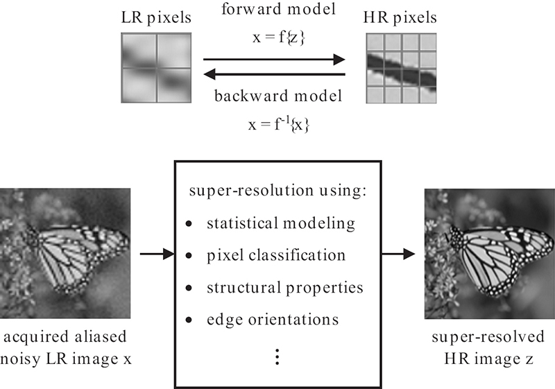
FIGURE 9.1
Single-frame SR block diagram. The forward model, f, is a mathematical description of the image degradation process exploiting the relationship between HR neighboring pixels. The inverse problem or backward model f−1is estimating the HR image from the low-quality captured image.
9.2.1 Single-Frame Super-Resolution
Single-frame SR approaches are widely applied solutions to the resolution enhancement problem, especially in cases where only one degraded low-resolution (LR) observation is available [17]. Single-frame SR approaches can also be referred to as image interpolation or reconstruction techniques and thus can be used interchangeably. Recovering a high-resolution image from an under-sampled (according to Nyquist limits [18]) and noisy observation is a highly ill-posed inverse problem. Thus, prior image models relating neighboring pixels or prior models learned through similar image patches are needed extra information that can aid in solving the inverse problem. A common approach among these SR techniques is that they take advantage of the relation between neighboring pixels of the same image to estimate the values of missing pixels. Figure 9.1 illustrates a general single-frame SR process where fand f− denote the forward and backward degradation process of the imaging system, respectively.
A well-known problem with common kernel-based super-resolution, such as bilinear and bicubic interpolation [19], is the blurring and blockiness effects of sharp edges. The blurring of sharp edges results from the inaccurate kernel resizing to adapt to the edge sharpness. The edge blockiness, also known as staircase effects, is mainly due to the failure of the filter to adapt to various edge orientations. Reference [20] proposed an edge-directed interpolation method that uses local covariance estimates of the input LR frame to adapt interpolation coefficients to arbitrarily oriented edges of the reconstructed HR image. This method is motivated by the geometric regularity property [21] of an ideal step edge. Recently, Reference [22] presented a new edge-directed interpolation approach that uses multiple low resolution training windows to reduce the covariance mismatch between the LR and HR pixels. Reference [23] proposed a smart interpolation method that uses anisotropic diffusion [24], a technique aiming at reducing noise and enhancing contrast without significantly degrading edges and objects in an image. References [25], [26], [27], [28], and [29] proposed SR methods based on the optimal recovery principle, which model the local image regions using ellipsoidal signal classes and adapts the interpolating kernels accordingly. Another model-based SR approach [30] is based on multi-resolution analysis in the wavelet domain, where the statistical relationships between coefficients at coarser scales are modeled using hidden Markov trees to predict the coefficients on the finest scale. Finally, learning-based SR approaches recover missing high-frequency information in an image through matching using a large image database [31], [32], [33], [34].
Many single-frame SR methods are computationally efficient. However, super-resolving from a single low-resolution image is known to be a highly ill-posed inverse problem due to the low number of observations relative to the large number of missing pixels/unknowns. Thus, the gain in quality in the single-frame SR approach is limited by the minimal number of information provided to recover missing details in the reconstructed HR signal.
9.2.2 Multi-Frame Super-Resolution
Multi-frame SR techniques offer a better solution to the resolution enhancement problem by exploiting extra information from several neighboring frames in a video sequence. In a multi-frame acquisition system, the subpixel motion between the camera and object allows the frames of the video sequence to contain oversampled similar information that make the reconstruction of an HR image possible.
This chapter focuses on multi-frame SR techniques that enhance the resolution of images by combining information from multiple low-resolution (LR) frames of the same scene to estimate a high-resolution (HR) unaliased and sharp/deblurred image under realistic bandwidth requirements and cost-effective hardware [6]. Interest in multi-frame super-resolution re-emerged in the recent years mainly due to the use of multi-frame image sequences, which can take advantage of additional spatio-temporal information available in the video content, and the increase of hardware computational power and advancement of display technologies, which make SR applications possible. Figure 9.2 presents a block diagram showing a multi-frame SR estimation process using multiple degraded LR frames, with subpixel shifts, to estimate one HR reference frame. The figure also shows the LR pixels registered relative to a common HR reference grid to further visualize the number of pixels used in the process of estimating the missing pixels in the SR image.
Since Reference [35] first introduced the multi-frame image restoration and registration problem/solution, several multi-frame SR approaches have been proposed in the past two decades. These multi-frame SR approaches are described and broadly categorized according to their methods of solution into Bayesian, regularized norm minimization, fusion-restoration (FR), and non-iterative fusion-interpolation (FI) approaches. Bayesian maximum a posteriori (MAP) solutions have gained great attention and proved to be effective due to the inclusion of a priori knowledge about the HR estimate and inherent probabilistic formulation of the relation between the LR observations and the HR image [36], [37], [38], [39]. Regularized norm minimization solutions aim at minimizing an error term with some smoothness regularization assumption on the HR estimate [40], [41], [42]. It was shown in Reference [42] that the l1-norm minimization approach is the most robust to errors in the system and that the bilateral total variation regularization function gave the best performance in terms of robustness and edge preservation. The two-step fusion-restoration (FR) SR estimation methods [40], [42] were devised in order to decrease the computational requirements and to increase the robustness to outliers. The FR methods employ a non-iterative fusion step, which includes a one-step registration process, and a restoration step, which simultaneously deblurs and denoises the fused image by minimizing an error function with or without a specific regularization term. The non-iterative fusion-interpolation (FI) SR approaches [43], [44] are composed of a fusion step and a non-iterative reconstruction step using kernel-based interpolation, which is inherently efficient in nature; however, these non-iterative methods can result in lower visual quality than the iterative methods as discussed later in this chapter. All the previous methods consider the subpixel motion between the observations to recover missing information by solving the SR problem.
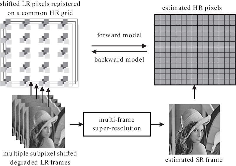
FIGURE 9.2
Multi-frame SR block diagram.
9.3 Multi-Frame Super-Resolution Observation Model
Multi-frame reconstruction techniques, as described earlier in Section 9.2.2, reduce the sensitivity of the SR inverse problem solution to some given LR observation measures by exploiting extra information from several neighboring frames in a video sequence. A necessary assumption for multi-frame SR solutions to work is the existence of subpixel shifts between the observed LR frames. Due to these fractional pixel shifts, registered LR samples will not always fall on a uniformly spaced HR grid, thus providing oversampled information necessary for solving the SR inverse problem. The LR pixels in the data acquisition model are defined as a weighted sum of appropriate HR pixels. The weighting function, also known as the system degradation matrix, models the blurring caused by the point spread function (PSF) of the optics. An additive noise term can be added to compensate for any random errors and reading sensor noise in the acquisition model. Assuming that the resolution enhancement factor is constant and the LR frames are acquired by the same camera, it is logical to consider the same PSF and statistical noise for all the LR observations. Taking into consideration all these assumptions, a common observation model for the SR problem is formulated.
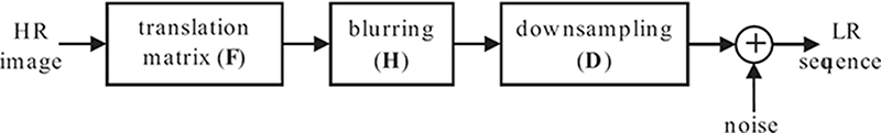
FIGURE 9.3
Multi-frame SR observation model.
Consider K low-resolution frames yk, for k = 1,2,...,K, each arranged in lexicographical form of size N1N2× 1 pixels. Let L1 and L2 be the resolution enhancement factors in the horizontal and vertical directions, respectively. For simplicity, it is assumed here that L = L1 = L2. The values of the pixels in the kth low-resolution frame of the sequence can be expressed in matrix notation as
where z represents the lexicographically ordered undegraded HR image of size N × 1 for N = L2N1N2, and n is the additive noise modeled as an independent and identically distributed (i.i.d.) Gaussian random variable with variance . In Equation 9.1, the degradation matrix is represented by Wk = DHFk, where Fk is the warping matrix of size N ×N, the term H denotes the blurring matrix of size N × N representing the common PSF function, and D is the decimation matrix of size N1N2× N.
Let y be the observation vector composed of all the LR vectors yk, for k = 1,2,...,K, concatenated vertically. The pointwise notation counterpart of Equation 9.1 for the mth element of yk is given by
where nm represents the additive noise and wm,r represents the contribution of zr (which is the rth HR pixel in z), to ym (which is the mth LR pixel in the observation vector y). Figure 9.3 illustrates the SR observation model for acquiring the LR frames.
9.4 Super-Resolution Problem Formulation
The formulation of the existing solutions for the SR problem usually falls into three main categories:
The Bayesian maximum likelihood (ML) methods and maximum a posteriori (pMAP) methods. The former ones produce a super-resolution image that maximizes the probability of the observed LR input images under a given model, whereas the latter ones aim at stabilizing the ML solution under noisy conditions by making explicit use of prior HR information.
The regularized-norm minimization methods produce an SR image by minimizing an error criteria (lp-norm) with a regularization term. Efficient methods emerged from this category by swapping the order of the warping and blurring operators in the observation model to fuse the images into one HR grid followed by an iterative regularized optimization solution. An example is the fusion-restoration class of SR methods, as discussed in Section 9.7.2.
The non-iterative kernel-based methods, also referred to as fusion-interpolation (FI) methods, merge all the observations on a common HR grid and solve for the best interpolation through adaptive kernel design techniques. This category is inherently computationally efficient since it is non-iterative in nature.
9.4.1 Bayesian Super-Resolution Formulation
Bayesian MAP-based estimators are common solutions for the SR problem since they offer fast convergence and high-quality performance [36], [37], [38], [39]. In Bayesian SR solutions all parameters or unknowns (that is, HR image, motion parameters, and noise) and observable variables (that is, the LR observations) are assumed to be unknown stochastic quantities with assumed probability distributions based on subjective beliefs. In the following formulation of the MAP solution, the motion parameters are assumed to be known for simplicity. For example, in cases of compressed video content the motion vectors can be retrieved from the headers of the bitstream (note that motion estimation is a mature field of research with many proposed accurate methods). In order to estimate the HR image z, a Bayesian MAP estimator is formed given the low-resolution frames yk, for k = 1,2,...,K, and appropriate prior. The HR estimate can be computed by maximizing the a posteriori probability Pr(z|, or by minimizing the log-likelihood function as follows:
Using Bayes rule and assuming that the LR observations yk are statistically independent of z, the problem reduces to
Now solving for an accurate HR estimate in Equation 9.4 is highly dependent on the prior HR image density Pr(z) and the conditional LR density Pr({yk}|z) models. Note that when dropping the prior HR probability model in Equation 9.4, the MAP optimization problem reduces to an ML estimation problem that is highly unstable under small errors in the parameters of the acquisition model and noisy conditions [37]. It has been widely used in Bayesian SR formulation literature [36], [37], [38], [39], [45], [46], [47], [48], [49], [50], [51], [52] that the noise model is assumed to be a zero mean Gaussian. From Equation 9.4, and given that the elements of nk are i.i.d Gaussian random variables, the conditional probability distribution can be modeled as follows:
where is the noise variance. The problem of determining which HR image prior model is the best for a particular HR reconstruction is still an open problem widely targeted by various existing literature [6], [53]. However, a common approach followed by existing MAP-based SR solutions is the assumption of smoothness constraints on the HR priors within homogeneous regions [36], [37], [54], [55]. These priors can generally be modeled as
where Q represents a linear high-pass operator that penalizes the estimates that are not smooth and λ controls the variance of the prior distribution. In References [36] and [37], these piecewise smoothness priors in Equation 9.6 take the form of Huber-Markov random fields that are modeled as Gibbs prior functional according to Reference [56]. Then, the prior model can be written as follows:
where Cz is the covariance of the HR image prior model imposing piecewise smoothness constraints between neighboring pixels. Thus, with the smoothness prior model (Equation 9.7) and mutually independent additive Gaussian noise on the prior error model (Equation 9.5), the MAP SR estimation problem can be formulated by minimizing the following convex cost function with a unique global minimum:
where Wk is the degradation matrix for frame k, the term denotes the noise variance, z is the HR frame in lexicographical form, and yk are the observed LR frames in vector form. Thus, the MAP estimator can be reformulated as a least-squares error minimization problem, which in matrix notation is the l2-norm square of the error vector, with a smoothness regularization constraint, given by
where is the square of the l2-norm and Cη is the i.i.d. Gaussian noise covariance matrix equal to . The λ in the second term is a regularization weighting factor, and Г(z) is a smoothness regularization constraint in function of the SR image prior.
9.4.2 Regularized-Norm Minimization Formulation
Here, an SR image is estimated by following a regularized-norm minimization paradigm [40], [41], [42], [57]. Then, in an underdetermined system of equations (Equation 9.1), estimating the HR image z given a sequence of LR observations yk, for k = 1,2,...,K, is commonly formulated as an optimization problem minimizing an error criteria and a regularization term. Thus, the SR optimization problem can be written as
where the cost function f(z) has the following form:
In the above equation, E(·) is the error term in function of yk and z. The weighting factors γ and λ are constant tuning parameters. The regularization term Г(·), which is in function of the HR image only, is designed to preserve important image content or structures, such as edges and objects, and also to increase the robustness of the solution to outliers and errors in the system. Unlike MAP-based algorithms, such as the one presented in Section 9.4.1, there is no a priori assumption made about the distribution function of the reconstructed HR image. Reference [42] proved that an l1-norm imposed on the error residual is the most robust solution against outliers. Also in Reference [42], different regularization terms are considered for best performance in terms of robustness and edge preservation. Therefore, a cost function formulation for the SR problem can be expressed as follows:
where is the lp-norm raised to the power p = {1,2}. The weighting factor γ is set to for p = {1,2}, respectively. Previous SR solutions are based on the warp-blur observation model following Equation 9.1. Assuming a circularly symmetric blurring matrix and a translation or rotation type of motion, then the motion and blur matrices in Equation 9.1 can be swapped. Consequently, the observation model, referred to by the blur-warp model, can be deduced from Equation 9.1 by defining the degradation matrix as Wk = DFkH, where Fk is the warping matrix of size N × N, the term H denotes the blurring matrix of size N × N representing the common PSF function, and D is the decimation matrix of size N1N2× N. The question as to which of the two models (blur-warp or warp-blur) should be used in SR solutions is addressed in Reference [58]. Following this blur-warp observation model, a fast implementation of the regularized-norm minimization solution, referred to as the fusion-restoration (FR) approach, can be achieved by solving for a blurred estimate of the HR image followed by an interpolation and deblurring iterative step. Often, the blurred HR estimate is a non-iterative approach composed of registering all the LR observations relative to the HR grid and estimating the HR pixel by using an average or median operator of the LR pixels at each HR location [40], [41], [42]. The formulation of this FR approach will be discussed in Section 9.7.2.

FIGURE 9.4
The blur-warp observation model for multi-frame SR.
9.4.3 Non-Iterative Kernel-Based Formulation
In the category of non-iterative kernel-based SR solutions, following the blur-warp observation model, all the LR observations are registered and merged on a common HR grid and non-iterative kernel-based solutions solve for the best estimate through adaptive kernel design techniques. The blur-warp acquisition model can be visualized as a non-uniform sampler (U = DFk) applied on the blurred HR estimate zb as shown in Figure 9.4.
A locally adaptive approach using such SR estimators is described in References [43] and [44], where the fused LR samples are processed using a moving observation window to estimate the interpolation kernel and an estimation window to apply the designed kernel on the spanned LR observed samples to estimate the missing HR pixels. Figure 9.5 illustrates the non-iterative estimation approach using locally adaptive convolution kernel processing.
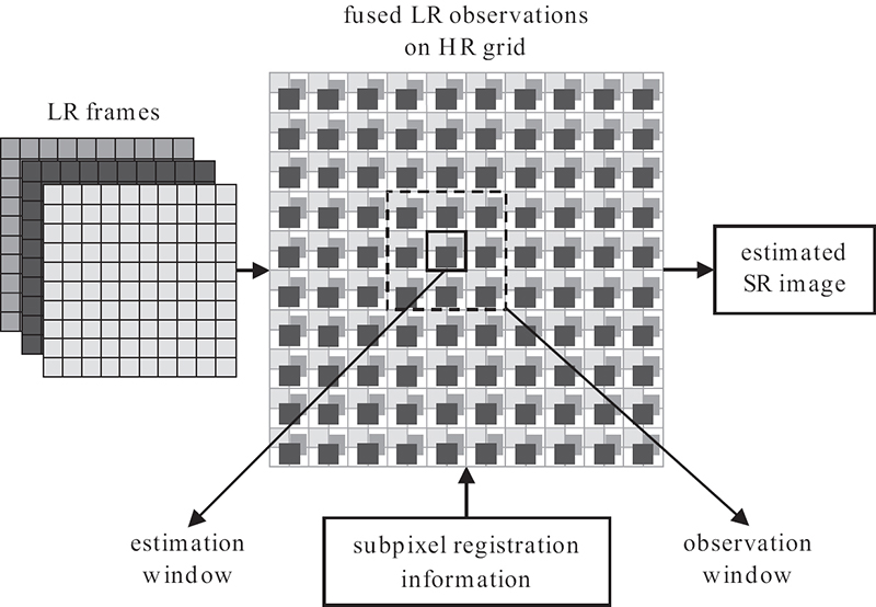
FIGURE 9.5
Non-iterative kernel-based SR.
From Figure 9.5, consider that the observation window is of size Wx × Wy pixels on the HR grid and spans P = KWxWy/L2 LR pixels denoted by vector Gi, and the estimation window is of size Dx × Dy pixels on the HR grid and spans DxDy estimated SR pixels denoted by vector Di, where i is the location of the respective window index. Estimating a local set of SR pixels can then be achieved by simply filtering the vector Gi by its locally designed kernel coefficients Wi, following Di = Wi.Gi. In Reference [43], the interpolation kernel coefficients are designed by minimizing the mean square error of Di− WiGi. Solving for the optimal weights of the matrix Wi for each partition reduces to an adaptive Wiener filter solution for the considered observed LR pixels in the window. In References [44] and [59], the weights of the Wiener filter are defined as
where and . Thus, the determination of the weighting coefficients in Equation 9.13 requires the unknown HR image that can be either modeled parametrically or by training data. To avoid training, a parametric modeling approach can be adopted as described in Reference [43]. This category of SR estimation is inherently computationally efficient since it is non-iterative in nature.
9.4.4 Super-Resolution Solutions in Practice
Existing SR approaches suffer from extremely high computational requirements due to the high dimensionality in terms of large number of unknowns to be estimated in the solution of the SR inverse problem. Generally, MAP-based SR methods are computationally expensive, but can converge to a high-quality solution. Even for solutions with fast convergence rates, commonly used Bayesian approaches are conditioned on the number of different LR observations and the HR image prior statistical model that can lead to very high computational requirements even for small image estimates. To reduce the computations required for the regularized norm minimization SR solutions, the fusion-restoration (FR) methods register and merge all the LR observations on one HR grid before using an iterative regularized minimization reconstruction process. However, these solutions are still computationally intensive due to the high dimensionality of the problem with good reconstruction quality. Moreover, the non-iterative fusion-interpolation (FI) SR approaches, also referred to as kernel-based SR, are inherently less computationally intensive but suffer from limited reconstruction quality depending on their assumed statistical model. Learning-based SR approaches recover missing high-frequency information in an image through matching using a large image database of training sets. The drawbacks of these methods is the requirement of large representative training sets that are targeted toward example-based and specific applications. For example, the MAP-based SR approach in Reference [37] requires a total of approximately 395 ×106 multiplication and addition operations to estimate an HR image with 256 × 256 pixels from 16 LR frames of size 64 × 64 pixels with translational motion and noise. Also, for the same problem, the FR-based SR method in Reference [42] requires approximately a total of 200 × 106 multiplication and addition operations. Additionally, the inherently faster non-iterative FI-based SR approach in Reference [43], with parameters set as Wx = Wy = 12, Dx = Dy = 4, and ρ = 0.75, requires 72 × 106 multiplication and addition operations but suffers from a limited reconstruction quality.
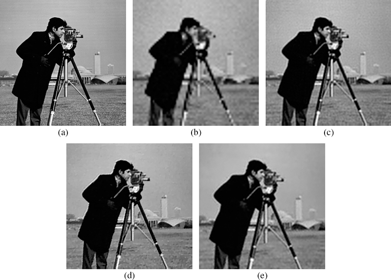
FIGURE 9.6
Super-resolved 256 × 256 HR Cameraman image obtained using sixteen 64 × 64 low-resolution images with noise standard deviation σn = 4: (a) original image, (b) bicubic interpolation with PSNR = 22.44 dB, (c) baseline MAP-SR with PSNR = 25.67 dB, (d) baseline FR-SR with PSNR = 25.73 dB, and (e) non-iterative FI-SR with PSNR = 24.11 dB.
Figure 9.6 compares the visual quality of the HR estimates generated using various SR solutions described in References [37], [42], and [43]. As it can be seen, the MAP-based [37] and the FR-based [42] result in a noticeably sharper image and approximately 2 dB increase in PSNR compared to the FI-based SR approach [43]. Given these results, the following sections present a new trend of efficient selective quality-preserving SR techniques that are driven by perceptual modeling of low-level features.
9.5 Perceptually Driven Efficient Super-Resolution
The high dimensionality of the SR image reconstruction problem demands high computational efficiency to be deemed of any practical value. As described in Section 9.4, many powerful iterative solutions were proposed to reduce the complexity and increase the stability of solving a very large system of linear equations. Although these SR methods are theoretically justifiable and presented reliable results in terms of image quality and robustness, still at each iteration all the pixels are processed on an HR grid inclusively and thus they still suffer from high dimensionality in solving the inverse problem. As a consequence, a selective perceptually driven efficient (SELP) SR framework, that takes into account the preservation of perceptual quality and the reduction of computational efficiency, has been introduced to reduce the dimensionality of existing iterative SR techniques. The perceptual SR approach is selective in nature; only a limited set of perceptually significant pixels, detected through human perceptual and/or attentive modeling, are super-resolved.
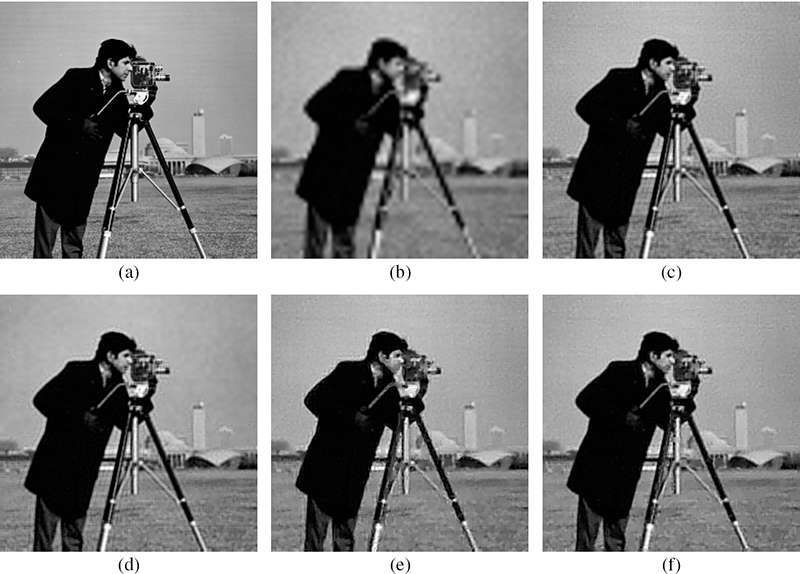
FIGURE 9.7
Super-resolved 256 × 256 HR Cameraman image obtained using sixteen 64 × 64 low-resolution images with noise standard deviation σn = 10: (a) original image, (b) bicubic interpolation, (c) baseline MAP SR, (d) SELPMAP SR, (e) gradient-detector with block-based mean thresholds (G-MAP) SR, and (f) entropy-detector with block-based mean thresholds (E-MAP) SR.
Early attempts on selective SR processing, as presented in References [10] and [11], used a non-perceptual gradient-based approach in order to detect active pixels that are signifi-cant for SR processing. Although the gradient-based approach (and other similar high-frequency detection-based approaches) resulted in savings, it suffered from a significant drawback, consisting of using a different threshold on the gradient for different images in order to be able to detect the pixels of interest and achieve good performance. This is not practical as it requires tweaking the gradient threshold for each image differently. Furthermore, general high-frequency detection methods, such as gradient or entropy based, do not incorporate any perceptual weighting and cannot automatically adapt to an image’s local high-frequency content that is perceptually relevant to the human visual system (HVS). Thus, in the SELP SR method [12], [13], a set of perceptually significant pixels is determined adaptively using an automatic perceptual detection mechanism that proves to work over a broad set of images without any manual tuning.
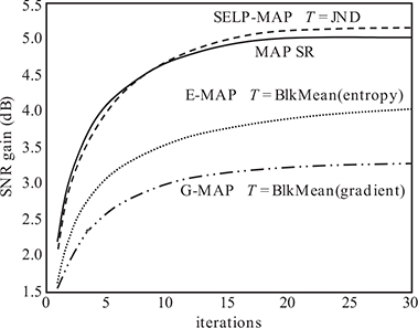
FIGURE 9.8
SNR comparison of the baseline MAP SR, SELP-MAP SR, G-MAP SR with block mean thresholds, and E-MAP SR approaches with block mean thresholds using sixteen 64 × 64 low-resolution images with noise standard deviation σn = 10 for the 256 × 256 Cameraman image.
The problem of devising automatic detection thresholds that can adapt to local image content perceptually is of major importance. Figures 9.7 and 9.8 demonstrate the superior performance of perceptual automatic thresholds, such as the SELP SR algorithm of References [12] and [13], and the one discussed in the following section, over the simple non-perceptual gradient and entropy-based approaches. To avoid the impractical manual tweaking of the detection thresholds for each image differently and to eliminate global thresholding that does not adapt to local image features and which was shown in Reference [11] to require manual tweaking to lead to good performance, the local non-perceptual detection thresholds are computed as the mean value corresponding to the magnitude of the gradient or entropy of each block of 8 × 8 pixels. That is, the detection mechanism in Reference [11] is replaced by locally thresholding the magnitude of the gradient (G-MAP), and locally thresholding the entropy (E-MAP).
Figure 9.7 clearly demonstrates the superior perceptual quality of the SELP SR method (Figure 9.7d) as compared with the non-perceptual methods, including the gradient-based (Figure 9.7e) and the entropy-based (Figure 9.7f) methods. Compared to the gradient-based and the entropy-based MAP SR methods, the SELP-MAP method results in a better reconstruction of edges, as it can be seen around regions such as the tripod of the camera and the face of the cameraman. Furthermore, Figure 9.8 illustrates the significant increase in SNR gains per iteration using the SELP-MAP method compared to the gradient-based and entropy-based MAP SR methods. It also shows that the SELP-MAP and the baseline MAP SR algorithms have similar performance.
9.5.1 Selective Perceptual Super-Resolution Framework
A block diagram of the SELP-SR estimation framework is shown in Figure 9.9. Initially, a rough estimate z0 of the high-resolution image is obtained by either interpolating one of the LR images in the observed sequence or by fusing all the LR frames on one HR grid (also referred to as the shift-and-add technique). Other techniques, such as learning-based approaches [31], [32], [33], can also be used to produce initial estimates. At each iteration and for each estimated HR image, active pixels are detected based on the human visual detection model described in Section 9.5.2. Then, only these perceptually active pixels are updated by the SR estimation algorithm, which is based generally on minimizing an SR cost function. As a result, at each iteration, only a subset of pixels (that is, the active pixels) is selected for the SR processing phase. The algorithm stops whenever the change between the current HR estimate and the previous one is less than a small number e, or whenever the total number of specified iterations is reached. Only the selected perceptually active pixels need to be included in computing the change in the estimated SR frames between iterations; the other pixels remain unchanged. The SELP SR framework is very flexible in that any iterative SR estimation algorithm can be easily integrated in the SELP system.

FIGURE 9.9
Flowchart of the selective perceptual SR framework.
9.5.2 Perceptual Contrast Sensitivity Threshold Model
Neurons in the primary visual cortex of the human visual system (HVS) are sensitive to various stimuli of low-level features in a scene, such as color, orientation, contrast, and luminance intensity [60]. The luminance sensitivity also referred to as light adaptation is the discrimination of luminance variations at every light level. Moreover, the contrast sensitivity is the response to local variations of luminance to the surrounding luminance [60]. Limits on the human visual sensitivity to low-level stimuli, such as light and contrast, are converted to masking thresholds that are used in perceptual modeling. Masking thresholds are levels above which a human can start distinguishing a significant stimulus or distortion [61]. Thus, the human visual detection model discriminates between image components based on contrast sensitivity of local information to their surroundings. In References [12] and [13], the SELP SR scheme attempts to exclude less significant information from SR processing by exploiting the masking properties of the human visual system through generating contrast sensitivity detection thresholds. The contrast sensitivity threshold is the measure of the smallest contrast, or the so-called just noticeable difference (JND), that yields a visible signal over a uniform background.
Digital natural images can be represented using linear weighted combinations of cosine functions through the discrete cosine transform (DCT). This is exploited in the lossy JPEG standard and many other image compression algorithms, including lossless ones. The models presented in References [62] and [63] derive contrast sensitivity thresholds and contrast masking thresholds for natural images in the DCT domain. The contrast sensitivity model considers the screen resolution, the viewing distance, the minimum display luminance Lmin, and the maximum display luminance Lmax. The contrast sensitivity thresholds are computed locally in the spatial domain using a sliding window of size Nblk × Nblk. The obtained thresholds per block will be used to select the pixels to be super-resolved for each HR estimate. The model, described in this section, involves first computing the contrast sensitivity threshold t128 for a uniform block having a mean grayscale value equals to 128, and then obtaining the threshold for any block having arbitrary mean intensity using the approximation model presented in Reference [63].
The contrast sensitivity threshold t128 of a block in the spatial domain is computed as
where Mg is the total number of grayscale levels (that is, Mg = 255 for eight-bit images), and Lmin and Lmax are the minimum and maximum display luminances, respectively. The threshold luminance T is evaluated based on the parametric model derived in Reference [62] using a parabolic approximation, where T = min(10g0,1, 10g1,0) and the terms g0,1 and g1,0 are defined as follows:
where wx and wy denote the horizontal width and vertical height of a pixel in degrees of visual angle, respectively. The term Tmin denotes the luminance threshold at the frequency fmin, where the threshold is minimum, and K determines the steepness of the parabola. The parameters Tmin, fmin, and K are the luminance-dependent parameters of the parabolic model and are computed as follows [62]:
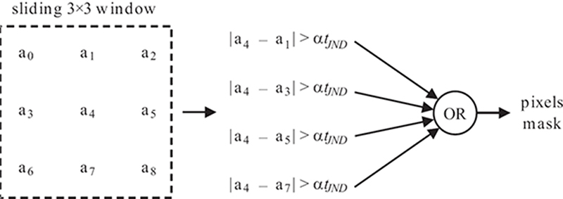
FIGURE 9.10
Generation process of the SELP mask.
In Reference [62], the values of the constants in Equations 9.17 to 9.19 are set as LT = 13.45cd/m2, S0 = 94.7, αT = 0.649, αf = 0.182, f0 = 6.78 cycles/deg, Lf = 300cd/m2, K0 = 3.125, αK = 0.0706, and LK = 300cd/m2. For a background value of 128, the local background luminance is computed as
where Lmin and Lmax denote the minumum and maximum luminance of the display, respectively. Once the threshold t128 at a grayscale value 128 is calculated using Equation 9.14, the just noticeable difference (JND) thresholds for the other grayscale values are approximated using a power function [63] as follows:
where In1, n2 is the intensity level at pixel location (n1, n2) and aT is a correction exponent that controls the degree to which luminance masking occurs and is set to αT = 0.649, as given in Reference [63]. Note that if the block has a mean of 128, then tJND of Equation 9.21 reduces to t128 as expected.
A DELL UltraSharp 1905 FP liquid crystal display is used to show the images. For a screen resolution of 1280 × 1024, and for a measured luminance of Lmin = 0cd/m2 and Lmax = 175cd/m2, the threshold t128 is computed to be equal to 3.3092 for Nblk = 8.
9.5.3 Perceptually Significant Pixels Detection
The perceptual mask determines the significant pixels that need to be processed at each iteration of the SR algorithm. For each estimated HR image, the perceptual mask is generated based on comparisons with the computed JND thresholds tJND (Section 9.5.2) over a local block of size 8 × 8 pixels. Note that t128 is computed only once according to Equation 9.14 since it is a constant. Also, for all eight-bit images, the remaining tJND values, corresponding to the 255 possible mean intensity values (other than 128), can be precomputed and stored in a lookup table (LUT) in memory. For each image block, the mean of the block is computed and the corresponding tJND is simply retrieved from the LUT.
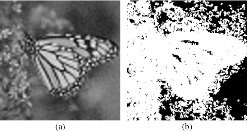
FIGURE 9.11
Illustration of the detected set of active pixels: (a) the blurred and noisy version of the 512 × 512 Monarch image and (b) the corresponding map Mp with white intensities denoting the active pixels selected using the perceptual mask.
As shown in Figure 9.10, after tJND is obtained, the center pixel of a sliding 3 ×3 window is compared to its four cardinal neighbors. If any absolute difference between the current center pixel and any of its four cardinal neighbors is greater than tJND, then the corresponding pixel mask is set to one indicating an active pixel. The remaining pixel mask locations are set to zero corresponding to non-active pixels. The sliding window will scan all the pixels of the HR image estimate to generate the perceptual mask. In general, the active locations consist of pixels in regions where edges are visible to the HVS. As a result, the perceptual mask signals a subset of pixels that are perceptually relevant for SR processing, resulting in significant computational savings. The SELP framework saves a significant number of computations in the SR processing stage with minimal overhead of operations per pixel for generating the perceptual mask. Figure 9.11 shows an example of the perceptually active pixels that are obtained by applying the SELP mask to a blurred and noisy version of the 512 × 512 Monarch image.
9.6 Attentively Driven Efficient Super-Resolution
To further enhance the SELP SR framework, previous work [14], [15] showed that not all the detail pixels detected by the SELP algorithm are needed to preserve the overall visual quality of an HR image. It is known that the human visual system scans a visual scene through a small window, restricted by the foveal region, having high central resolution and degrading resolution toward the peripheries. A large field of view is processed by a number of fixation points, attended to with high visual acuity, connected by fast eye movements referred to as saccades. The ordered selection of these regions of interest is predicted according to a visual attention model by studying the eye movement sensitivity to top-down mechanisms, such as image understanding, and bottom-up salient image features, such as contrast of color intensity, edge orientations, and object motion [64], [65]. Given the fact that the attended regions are processed at high visual acuity, artifacts present in these regions are better perceived by the HVS than artifacts present in non-attended areas. In consequence, the observer’s judgment of image quality is prejudiced by distortions present in salient regions as shown in Reference [66]. Following this logic, saliency maps generated by visual attention modeling, can play a fundamental role in reducing the number of processed pixels of selective SR approaches. Hence, an attentive selective perceptual (AT-SELP) SR estimators, that exploit the human visual attention for processing the visual content, are introduced in References [14], [15], and [67]. Moreover, different low-level features influenced by visual attention models presented in References [68], [69], and [70] are studied to illustrate the efficiency and quality of the attentive SR framework.
9.6.1 Attentive-Selective Perceptual Super-Resolution Framework
A block diagram of the AT-SELP SR estimation framework is shown in Figure 9.12. Similarly as in Figure 9.9, at each iteration and for each estimated HR image, active pixels are detected based on the human visual detection model described in Sections 9.5.2 and 9.6.2. Then, only these perceptually active pixels are updated by the SR estimation algorithm which is generally based on minimizing an SR cost function as in Equation 9.10. As a result, at each iteration, only a subset of pixels (that is, the active pixels) is selected for the SR processing phase.
The first phase of the SR algorithm processes the perceptually active pixels determined by a contrast sensitivity mask Mp, as explained in Section 9.5.3. Then, in the second phase of the SR estimation, only the subset of active pixels that is determined to be salient by the selective attention mask Ma is further iterated upon. The process of updating the HR estimates of the perceptual/attentive active pixels continues until a maximum number of iterations is reached or the system stabilizes; that is, until |Ma·(zn+1 − zn)|/|Ma·zn| < ε in the attentive active region and |Mp·(zn+1 − zn)|/|Mp·zn| < s·ε in the perceptual non-attentive active region. Here, s is a scaling factor greater than 1 and ε is a predetermined threshold that represents the desired accuracy or quality of the SR algorithm. Only the selected perceptually active and salient attentive pixels need to be included in computing the change in the estimated SR frames between iterations; the other pixels do not change their values. It is necessary in the first phase of the algorithm to super-resolve the perceptually significant information of the non-attended regions to a certain acceptable quality level (s.ε) that will not attract and bias the HVS perception of the background quality, thus, leading to an acceptable homogeneous quality of the entire image. As a result, the salient regions are reconstructed with a higher visual acuity while maintaining a trade-off between smoothing the flat regions dominated by noise and sharpening the perceptually relevant edges.
9.6.2 Saliency-Based Mask Detection
Any saliency-based visual attention model, such as those in References [68], [69], and [70], can be adopted to detect the attentive mask Ma in the AT-SELP SR framework to further reduce the set of active pixels selected by the contrast sensitivity detector, thus reducing the computational complexity of the SR algorithms. Saliency maps S combine several low-level image features that compete to attract the human attention, providing measures of the level of attention at every point in the visual scene. After computing the saliency information at each point in the scene, the attentive mask Ma is generated by choosing the pixel locations corresponding to the highest τ% of the saliency map values. Existing saliency map generation techniques inspired by a hierarchical visual attention model (IT) [68], a foveated gaze attentive model (GAF) [69], and a frequency-tuned attention model (FT) [70] are detailed in this section for further comparisons and analysis in the AT-SELP SR framework.
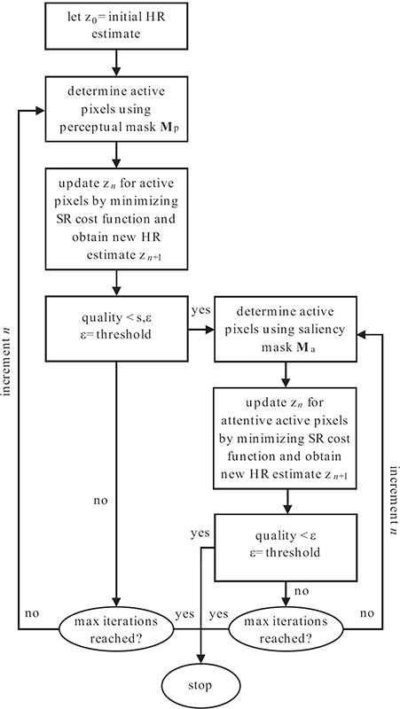
FIGURE 9.12
Flowchart of the AT-SELP SR framework.
9.6.2.1 Hierarchical Saliency Model
Reference [68] computes a hierarchical saliency map SIT using center-surround differences of intensity and orientation between different dyadic Gaussian scales. The input image I is subsampled into a dyadic Gaussian pyramid of four levels σ, obtained by progressively filtering and downsampling each direction separately. The intensity information is the image intensity values at each pyramid level, Iσ. The orientation information is calculated by convolving the intensity pyramid with Gabor filters as follows:
where Gψ(θ) is a Gabor filter with phase ψ = [0,π/2] and orientation θ = [0, π/4, π/2,3π/4]. The foveated visual perception and the antagonistic “center-surround” process are implemented as across-scale differences between fine levels c = {1,2} corresponding to center pixels, and coarse levels s = c + δ with chosen δ = {1,2} corresponding to surround pixels. The across-scale difference ⊖ is calculated by interpolation to the finer scale followed by point-by-point subtraction. Feature maps that signify the sensitivity of the HVS to differences in intensity and orientation are calculated as follows:
At this point, four intensity feature maps and sixteen orientation feature maps are created. Each group of feature maps is combined into two conspicuity maps through across-scale addition ⊕ by downsampling each map to the second scale of the pyramid followed by point-by-point addition. A map normalization operator is applied to scale the values of different ranges into a common fixed range [0, M]. The conspicuity maps for intensity and orientation are calculated as follows:
A saliency map is then calculated by averaging over the two normalized conspicuities as
Figure 9.13a shows the attentive mask Ma(IT) generated from the hierarchical saliency map with τ = 20%. The resulting attended regions are used in the AT-SELP method to promote the detected subset of attended pixels for further iterations or enhancement.
9.6.2.2 Foveated Saliency Model
A foveated visual attention model in Reference [69] is based on the analysis of the statistics of low-level features at the point of gaze in a scene. The saliency map SGAF is generated by a foveated combination of low-level image features, such as mean luminance, contrast, and bandpass outputs of both luminance and contrast. For an image patch of size M = M1 × M2, the mean luminance Ī is calculated as follows:
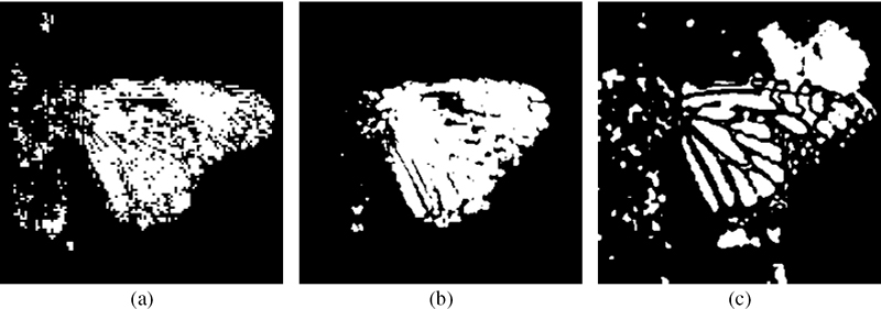
FIGURE 9.13
Illustration of the detected set of active pixels (20% of highest saliency values) for the blurred and noisy version of the 512 × 512 Monarch image shown in Figure 9.11 by generating and applying: (a) the hierarchical attentive mask Ma(IT), (b) the foveated attentive mask Ma(GAF), and (c) the frequency-tuned attentive mask Ma(FT). White intensities denote active pixels.
where Ii is the grayscale value of the pixel at patch location i, and wi is the raised cosine function given by
where is the radial distance of pixel location (xi, yi) from the center of the patch (xc, yc) and R is patch radius. Then, the root-mean-squared contrast C is computed as follows:
The bandpass of patch luminance features are computed by using Gabor kernels designed for different eccentricity values. Eccentricity values e, measured in degrees of visual angle, represent the distance needed to reach a particular patch. Then the bandpass-luminance for each patch is computed as Glum = max|Glum(e)*I(e)|, where Glum(e) is the designed Gabor filter at eccentricity e. Similarly, the bandpass of patch contrast is computed using Ggrad = max|Ggrad(e) * |∇(I(e))||, where Ggrad(e) is the designed Gabor filter at eccentricity e of the image gradient |∇(I(e))|. More details on the Gabor filters design can be found in Reference [69]. The saliency map is then calculated by averaging all the computed image features after scaling them to a common fixed range [0, M]. Figure 9.13b shows the attentive mask Ma(GAF) generated from the foveated saliency map with τ = 20%.
9.6.2.3 Frequency-Tuned Saliency Model
Reference [70] proposed a frequency-tuned saliency approach, using difference of Gaussians (DoG) of luminance intensity, to generate saliency map information SFT. The bandpass filters using DoG are designed by properly selecting the standard deviation of the Gaussian filters targeting saliency generation. In Reference [70], the saliency map information (SFT) is generated by taking the magnitude of the differences between the image mean vector and Gaussian blurred version using a 5 × 5 separable kernel as follows:
where |·| is the norm operator, Iμ is the arithmetic mean pixel value of the image, and Iwhc is the Gaussian blurred version of the original image. Figure 9.13c shows an example of the attentive mask Ma(FT) to a blurred and noisy version of the 512 × 512Monarch image. Comparing the masks shown in Figures 9.13a to 9.13c and the perceptual mask (Mp) shown in Figure 9.11 reveals that the significantly lower number of active pixels is selected for SR processing using the attentive masking phase.
The existing visual attention approaches [68], [69] introduce a significant computational overhead for computing the saliency maps. These would be useful for the AT-SELP framework only if the saliency maps were already precomputed as part of another task (such as visual quality assessment for example). Such available saliency maps can then be exploited to improve the efficiency of the SR process. However, if these saliency maps were not available, generating those using the existing visual attention methods would not improve the SR process due to the high computational overhead that is introduced when computing these saliency maps. In order to tackle this issue and make the AT-SELP process feasible when saliency maps are not available, an efficient low-complexity JND-based saliency detector targeted toward efficient selective SR was recently proposed in Reference [67].
9.7 Perceptual SR Estimation Applications
The perceptually driven SR frameworks (SELP, AT-SELP), previously discussed in Sections 9.5 and 9.6, are very flexible in that any iterative SR estimation algorithm can be easily integrated in the perceptually selective system. Hence, application of the selective perceptual (SELP) and the attentive selective (AT-SELP) SR framework to an iterative MAP-based SR method [37] and a FR-based SR method [42] are described below in Sections 9.7.1 and 9.7.2, respectively. The attentively or perceptually driven SR schemes result in significant computational savings while maintaining the perceptual SR image quality, as compared to the iterative baseline SR schemes [37], [42].
9.7.1 Perceptual MAP-Based SR Estimation
Existing Bayesian MAP-based SR estimators present high-quality estimation but suffer from high computational requirements [36], [37], [38], [39]. In order to illustrate the significant reduction in computations for MAP SR techniques, the popular gradient-descent optimization-based algorithm from Reference [37] is integrated into the attentive-perceptual selective SR framework (SELP, AT-SELP).
In Reference [37], a uniform detector sensitivity is assumed over the span of the detector degradation model, then the point spread function (PSF) H in the observation model (Section 9.3) is represented using an averaging filter. Following the Bayesian MAP-based SR formulation in Section 9.4.1, the regularization smoothness constraint term (in the cost function of Equation 9.9) is represented in Reference [37] by , where Cz is the covariance of the HR image prior model imposing a piecewise smoothness relationship between neighboring pixels in z as follows [37]:
where λ is scaling factor controlling the effect of rapidly changing features in z, and zj is the pixel at the jth location of the lexicographically ordered vector z. The coefficients di,j, which express a priori assumption about the relationship between neighboring pixels in z, are defined as follows [37]:
In the AT-SELP-MAP SR scheme, the gradient descent minimization procedure is applied selectively and only to pixels that are determined to be perceptually significant by the attentive-perceptual detectors (Sections 9.5.3 and 9.6.2). Following the steepest descent solution in the perceptually driven framework, the HR image is estimated using Equation 9.8 as follows [37]:
where M represents the attentive-perceptual mask for selecting active pixels at every iteration of the SR process. Note that the initial HR image estimate is an interpolated version of one of the LR frames. The elements in M take binary values, where ones indicate active pixels that should be included in the SR update at the current iteration, whereas zero mask values indicate that the corresponding pixels are non-active and will not be processed in the current iteration.
9.7.2 Perceptual Fusion-Restoration SR Estimation
The efficient perceptually driven framework can be used in conjunction with the fusion-restoration (FR) SR algorithms. Reference [42] proposed a two-step algorithm by using first a non-iterative data fusion step followed by an iterative gradient-descent deblurring-interpolation step. This algorithm models the relative motion between low-resolution frames as translational and the point spread function (PSF) as an L1 × L2 Gaussian lowpass filter with a standard deviation equals to 1. Following the regularized-norm SR formulation in Section 9.4.2, a fast fusion-restoration implementation of the minimization solution (Equation 9.12) can be achieved by solving for a blurred estimate of the HR image followed by an interpolation and deblurring iterative step. An initial blurred version of the HR estimate zb is produced in the data fusion step by registration followed by a median operator of the LR frames on the HR grid, referred to as the “median shift and add” operator. As for the regularization term in Equation 9.12, a bilateral total variation regularization that preserves edges is adopted as follows [42]:
where and shift the HR image z by l and m pixels in the horizontal and vertical directions, respectively, and R ≥ 1 represents several scales of shifting values. The weight α is applied as a decaying factor for convergence purposes, and is chosen between 0 ≤ α ≤ 1. The SR problem in Equation 9.12 reduces to deblurring and interpolating for the missing pixels in the initial HR estimate zb that is formulated as a regularized l1-norm minimization problem [42]. In the AT-SELP-FR SR scheme, the steepest descent minimization is applied selectively only to the active pixels identified by the perceptual detection schemes:
where βn is the step size in the direction of the gradient and λ is a regularization weighting factor. Matrix A is an N × N diagonal matrix with diagonal values equal to the square root of the number of measurements that contribute to make each element of zb. Also, and define a shifting effect in the opposite directions of and . The term M represents the perceptually attentive masking that selects the active pixels that are processed at each iteration, thus reducing the computations required in Reference [42].
9.7.3 Perceptually Driven SR Results
The performance of the efficient perceptually driven SR framework is assessed using a set of test images shown in Figure 9.14. The images used in this experiment include Cameraman, Lena, and Clock from the USC image database [71], and Monarch from the LIVE image database [72], as shown in Figure 9.14. These images, all of the size of 256 × 256 pixels, differ in their characteristics. For example, the Clock and Monarch images contain many smooth regions, while the Cameraman and Lena images have more edges and texture variations. Moreover, the Lena image can be used to demonstrate the application of SR in face recognition applications.
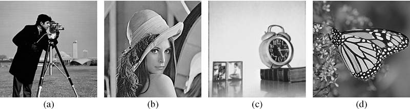
FIGURE 9.14
Original 256 × 256 test images: (a)Cameraman, (b)Lena, (c)Clock, and (d)Monarch.

FIGURE 9.15
Comparison between the baseline MAP, SELP-MAP, and the AT-SELP-MAP SR estimators using sixteen 64 × 64 LR images, resizing factor L = 4, and noise variance = 16 for the ninth frame of the 256 × 256 Cameraman sequence: (a) SNR gain per iteration and (b) number of processed pixels per iteration.
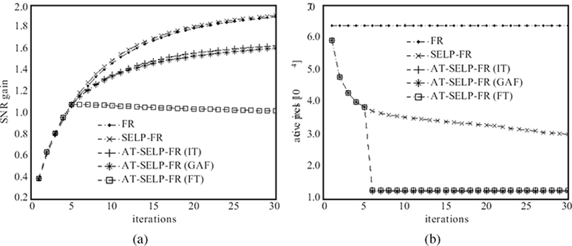
FIGURE 9.16
Comparison between the baseline FR, SELP-FR, and the AT-SELP-FR SR estimators using sixteen 64 × 64 LR images, resizing factor L = 4, and noise variance = 16 for the ninth frame of the 256 × 256 Cameraman sequence: (a) SNR gain per iteration and (b) number of processed pixels per iteration.
A sequence of LR images is generated from a single HR image by passing the HR image through the SR degradation model described in Section 9.3 to generate a sequence of blurred, shifted, and noisy LR images. Then, for a resolution factor of four, the degradation process is applied by randomly shifting the reference 256 × 256 HR image in the horizontal and vertical directions, blurring the shifted images with a lowpass filter of size 4 × 4, and subsampling the result by a factor of four in each direction to generate sixteen 64 × 64 LR frames. The blur filters are modeled as an average filter and as a Gaussian filter with standard deviation of one for the MAP-based [37] and the FR-based [42] SR observation models, respectively. Then, an additive Gaussian noise of variance = 16 is added to the resulting LR sequence. Figure 9.3 depicts the simulated sequence generation process.
The attentive-selective perceptual MAP-based super-resolution and attentive-selective perceptual fusion-restoration super-resolution schemes referred to as AT-SELP-MAP [15] and AT-SELP-FR [14], respectively, are compared with their existing non-selective counterparts MAP-SR [37] and FR-SR [42], as well as the selective SR counterparts SELP-MAP and SELP-FR [12], [13]. The simulation parameters of the compared MAP-based SR methods are set to λ = 100, ε = 0.0001, and s = 100, and a maximum of twenty iterations are performed. On the other hand, the simulation parameters of the compared FR-based SR methods are set to R = 2, α = 0.6, λ = 0.08, and β = 8, ε = 0.0001, s = 120, and a maximum of thirty iterations are performed. The parameter τ of the saliency map detection is set to 20% to identify the attentive active pixels. Experimentally, percentage values between 20 and 40% offered promising results in terms of quality and computational efficiency trade-off. These numbers are plausible, since shifts of attention based on competing saliency results needs 30 to 70 ms [73]. Then, in a 30.33 ms time interval given to view one frame, assuming 30 fps video sequence, one can only perceive 20 to 40% of the salient regions. For the saliency mask detection schemes, different saliency maps generated from existing visual attention models presented in References [68], [69], [70] are also integrated and tested in the proposed AT-SELP SR framework.
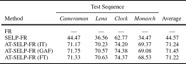
Figure 9.15 gives a quantitative comparison among the baseline MAP, SELP-MAP, and proposed AT-SELP-MAP SR methods using different saliency detection techniques applied to super-resolve the ninth frame of the simulated Cameraman LR sequence. Similarly, Figure 9.16 shows a quantitative comparison among the baseline FR, SELP-FR, and proposed AT-SELP-FR SR methods. Error measures, represented by the SNR gain per iteration, and the computational complexity, signified by the number of processed pixels per iteration, are presented in Figures 9.15, 9.16a, and 9.16b, respectively. It can be seen that in the case of baseline MAP and FR SR methods all the pixels are processed at each iteration for all the images (that is, for a 256 × 256 image, the total number of processed pixels is 65536 at each iteration). As shown in Figures 9.15b and 9.16b for the SELP-MAP and SELPFR SR methods, respectively, the number of processed pixels per iteration varies from one image to the other depending on the visual content. In Figures 9.15b and 9.16b, the visual attention processing takes effect around the fifth iteration, thus further reducing the detected active pixels processed. Due to the attentive selectivity, the AT-SELP SR framework presents considerable savings in terms of the number of processed pixels, leading to a significant reduction in computational complexity. Comparing the SNR measures in Figures 9.15a and 9.16a, it can be easily seen that the Ma(IT) mask integrated into the ATSELP SR framework has the best error performance among the other implemented saliency mask detectors. Also, the efficient and simple saliency mask generator Ma(FT) adopted from Reference [70] does not enhance the overall quality of the SR estimate due to selecting objects and features in the image that are not relevant to SR processing applications. Furthermore, the overall quantitative assessment is also shown in terms of PSNR measures in Tables 9.1 and 9.2.
Since the employed PSNR and SNR gain measures do not necessarily reflect the resulting visual quality [74], Figures 9.17 and 9.18 show the SR outputs obtained for the ninth frame of the simulated Cameraman sequence for all compared MAP-based and FR-based SR methods, respectively. Despite the fact that the AT-SELP-SR scheme processes significantly less pixels per iteration, it produces a comparable visual quality to the existing selective and non-selective [37], [42] SR schemes. Furthermore, Tables 9.3 and 9.4 show similar pixel savings achieved by the different visual attention methods when integrated in the AT-SELP SR framework. It is shown in Table 9.3 that up to 66% in pixel savings can be achieved by the AT-SELP-MAP SR over the baseline MAP SR, while around 31% in pixel savings is achieved over the efficient SELP-MAP SR. Table 9.4 shows that the proposed AT-SELP-FR framework saves around 71% in SR processing over the non-selective baseline-FR and around 44% in SR processing over the efficient SELP-FR SR.
TABLE 9.1
PSNR values in dBs of MAP-based SR methods for all test sequences using magnification factor L = 4 and noise variance = 16
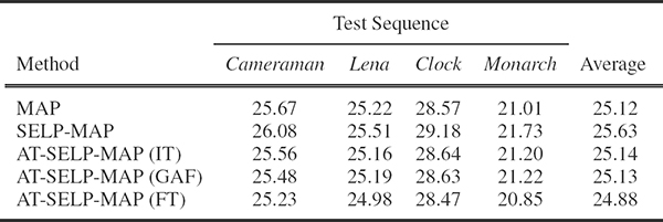
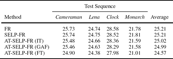
TABLE 9.2
PSNR values in dBs of FR-based SR methods for all test sequences using magnification factor L = 4 and noise variance = 16.
9.8 Conclusion
This chapter provided an overview of existing SR techniques, with a focus on perceptually driven multi-frame super-resolution (SR) techniques. The MAP-based SR methods, that are based on Bayesian formulations of the SR problem, strongly depend on prior HR information. The MAP SR approaches were shown to have a good reconstruction quality but with high computational requirements. The FR-based SR methods provide relatively efficient implementations of the regularized-norm minimization methods by reducing matrix operations and are more robust to errors.
This chapter also presented a new class of perceptually driven selective (SELP, AT-SELP) SR solutions that can reduce the computational complexity of iterative SR problems while maintaining the desired estimated HR media quality. It was shown that general high-frequency and edge detection methods, such as gradient-based or entropy-based methods, that do not incorporate any perceptual weighting, cannot automatically adapt to local visual characteristics that are perceptually relevant to the human visual system (HVS). Thus, the problem of devising automatic detection thresholds that can adapt to the local perceptually relevant image content is addressed. Due to human visual attention, not all the detail pixels detected by the contrast sensitivity threshold model are needed to preserve the overall visual quality of an HR image. Toward this goal, an efficient attentive-selective perceptual (ATSELP) SR framework jointly driven by human visual perception and saliency-based visual attention models, was presented. The effectiveness of the proposed attentive-perceptual framework in reducing the amount of SR processing while maintaining the desired visual quality was verified by investigating different saliency map techniques that combine several low-level features, such as center-surround differences in intensity and orientation, patch luminance and contrast, and bandpass outputs of patch luminance and contrast. The SELP and AT-SELP SR frameworks were shown to be easily integrated into a MAP-based SR algorithm as well as a FR-based SR estimator. Simulation results showed significant reduction on average in computational complexity with comparable visual quality in terms of subjectively perceived quality as well as PSNR, SNR, or MAE gains.
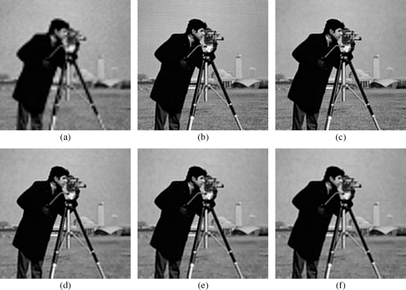
FIGURE 9.17
Super-resolved ninth frame of 256 × 256 HR Cameraman image obtained using sixteen 64 × 64 low-resolution images with = 16 and τ = 20%: (a) bicubic interpolation, (b) baseline MAP-SR, (c) SELP-MAP SR, (d) AT-SELP-MAP SR using hierarchical Ma(IT), (e) AT-SELP-MAP SR using foveated Ma(GAF), and (f) AT-SELP-MAP SR using frequency-tuned Ma(FT).
TABLE 9.3
Percentage of pixel savings of MAP-based SR methods for all test sequences using magnification factor L = 4 and noise variance = 16.
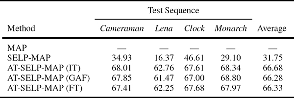

FIGURE 9.18
Super-resolved ninth frame of 256 × 256 HR Cameraman image obtained using sixteen 64 × 64 low-resolution images with = 16 and τ = 20%: (a) bicubic interpolation, (b) baseline FR-SR, (c) SELP-FR SR, (d) ATSELP-FR SR using hierarchical Ma(IT), (e) AT-SELP-FR SR using foveated Ma(GAF), and (f) AT-SELP-FR SR using frequency-tuned Ma(FT).
TABLE 9.4
Percentage of pixel savings of FR-based SR methods for all test sequences using magnification factor L = 4 and noise variance = 16.
References
[1] T. Akgun, Y. Altunbasak, and R. Mersereau, “Super-resolution reconstruction of hyperspectral images,” IEEE Transactions on Image Processing, vol. 14, no. 11, pp. 1860–1875, November 2005.
[2] T. Celik, C. Direkoglu, H. Ozkaramanli, H. Demirel, and M. Uyguroglu, “Region-based super-resolution aided facial feature extraction from low-resolution sequences,” in Proceedings of the IEEE International Conference on Acoustics, Speech, and Signal Processing, Philadelphia, PA, USA, March 2005, vol. 2, pp. 789–792.
[3] J. Kennedy, O. Israel, A. Frenkel, R. Bar-Shalom, and H. Azhari, “Super-resolution in PET imaging,” IEEE Transactions on Medical Imaging, vol. 25, no. 2, pp. 137–147, February 2006.
[4] M. Robinson, S. Farsiu, J. Lo, and C. Toth, “Efficient restoration and enhancement of super-resolved X-ray images,” in Proceedings of the IEEE International Conference on Image Processing, San Diego, CA, USA, October 2008, pp. 629–632.
[5] M. Mancuso and S. Battiato, “An introduction to the digital still camera technology,” ST Journal of System Research, vol. 2, no. 2, pp. 1–9, December 2001.
[6] S.C. Park, M.K. Park, and M.G. Kang, “Super-resolution image reconstruction: A technical overview,” IEEE Signal Processing Magazine, vol. 20, no. 3, pp. 21–36, May 2003.
[7] T. Komatsu, K. Aizawa, T. Igarashi, and T. Saito, “Signal-processing based method for acquiring very high resolution images with multiple cameras and its theoretical analysis,” IEE Proceedings on Communications, Speech and Vision, vol. 140, no. 1, pp. 19–24, February 1993.
[8] B.C. Tom, N.P. Galatsanos, and A.K. Katsaggelos, “Reconstruction of a high resolution image from multiple low resolution images,” in Super-Resolution Imaging, S. Chaudhuri (ed.), Boston, MA, USA: Kluwer Academic Publishers, 2001, pp. 73–105.
[9] Y. Wang, J. Ostermann, and Y.Q. Zhang, Video Processing and Communications. Boston, MA, USA: Prentice Hall, 2002.
[10] Z. Ivanovski, L. Karam, and G. Abousleman, “Selective Bayesian estimation for efficient super-resolution,” in Proceedings of the Fourth IEEE International Symposium on Signal Processing and Information Technology, Rome, Italy, December 2004, pp. 433–436.
[11] Z. Ivanovski, L. Panovski, and L.J. Karam, “Efficient edge-enhanced super-resolution,” in Proceedings of the 3rd International Conference on Sciences of Electronic, Technologies of Information and Telecommunications, Sousse, Tunisia, March 2005, pp. 35:1–5.
[12] R. Ferzli, Z. Ivanovski, and L. Karam, “An efficient, selective, perceptual-based super-resolution estimator,” in Proceedings of the IEEE International Conference on Image Processing, San Diego, CA, USA, October 2008, pp. 1260–1263.
[13] L. Karam, N. Sadaka, R. Ferzli, and Z. Ivanovski, “An efficient, selective, perceptual-based super-resolution estimator,” IEEE Transactions on Image Processing, 2011.
[14] N. Sadaka and L. Karam, “Efficient perceptual attentive super-resolution,” in Proceedings of the IEEE International Conference on Image Processing, Cairo, Egypt, November 2009, pp. 3113–3116.
[15] N. Sadaka and L. Karam, “Perceptual attentive super-resolution,” in Proceedings of the International Workshop on Video Processing and Quality Metrics for Consumer Electronics, Scottsdale, AZ, USA, January 2009.
[16] F. Liu, J. Wang, S. Zhu, M. Gleicher, and Y. Gong, “Visual-quality optimizing super resolution,” Computer Graphics Forum, vol. 28, no. 1, pp. 127–140, March 2009.
[17] J. van Ouwerkerk, “Image super-resolution survey,” Image and Vision Computing, vol. 24, no. 10, pp. 1039–1052, October 2006.
[18] A.K. Jain, Fundamentals of Digital Image Processing. Englewood Cliffs, NJ, USA: Prentice Hall, 1989.
[19] T. Lehmann, C. Gonner, and K. Spitzer, “Survey: Interpolation methods in medical image processing,” IEEE Transactions on Medical Imaging, vol. 18, no. 11, pp. 1049–1075, November 1999.
[20] X. Li and M. Orchard, “New edge-directed interpolation,” IEEE Transactions on Image Processing, vol. 10, no. 10, pp. 1521–1527, October 2001.
[21] S.G. Mallat, A Wavelet Tour of Signal Processing. New York, USA: Academic, 1998.
[22] W.S. Tam, C.W. Kok, and W.C. Siu, “Modified edge-directed interpolation for images,” Journal of Electronic Imaging, vol. 19, no. 1, pp. 013011:1–20, January 2010.
[23] S. Battiato, G. Gallo, and F. Stanco, “Smart interpolation by anisotropic diffusion,” in Proceedings of the International Conference on Image Analysis and Processing, Rome, Italy, September 2003, pp. 572–577.
[24] P. Perona and J. Malik, “Scale-space and edge detection using anisotropic diffusion,” IEEE Transactions on Pattern Analysis and Machine Intelligence, vol. 12, no. 7, pp. 629–639, July 1990.
[25] D. Muresan and T. Parks, “Adaptively quadratic (AQUA) image interpolation,” IEEE Transactions on Image Processing, vol. 13, no. 5, pp. 690–698, May 2004.
[26] D. Muresan and T. Parks, “Adaptive, optimal-recovery image interpolation,” in Proceedings of the IEEE International Conference on Acoustics, Speech, and Signal Processing, Salt Lake City, UT, USA, May 2001, vol. 3, pp. 1949–1952.
[27] D. Muresan and T. Parks, “Optimal recovery approach to image interpolation,” in Proceedings of the IEEE International Conference on Image Processing, Thessaloniki, Greece, October 2001, vol. 3, pp. 848–851.
[28] D. Muresan and T. Parks, “Demosaicing using optimal recovery,” IEEE Transactions on Image Processing, vol. 14, no. 2, pp. 267–278, February 2005.
[29] D. Muresan and T. Parks, “Prediction of image detail,” in Proceedings of the IEEE International Conference on Image Processing, Vancouver, BC, Canada, September 2000, vol. 2, pp. 323–326.
[30] K. Kinebuchi, D. Muresan, and T. Parks, “Image interpolation using wavelet based hidden Markov trees,” in Proceedings of the IEEE International Conference on Acoustics, Speech, and Signal Processing, Salt Lake City, UT, USA, May 2001, vol. 3, pp. 1957–1960.
[31] W. Freeman, T. Jones, and E. Pasztor, “Example-based super-resolution,” IEEE Computer Graphics and Applications, vol. 22, no. 2, pp. 56–65, March/April 2002.
[32] P. Gajjar and M. Joshi, “New learning based super-resolution: Use of DWT and IGMRF prior,” IEEE Transactions on Image Processing, vol. 19, no. 5, pp. 1201–1213, May 2010.
[33] Z. Xiong, X. Sun, and F. Wu, “Robust web image/video super-resolution,” IEEE Transactions on Image Processing, vol. 19, no. 8, pp. 2017–2028, August 2010.
[34] Y.W. Tai, W.S. Tong, and C.K. Tang, “Perceptually-inspired and edge-directed color image super-resolution,” in Proceedings of the IEEE Conference on Computer Vision and Pattern Recognition, New York, USA, June 2006, vol. 2, pp. 1948–1955.
[35] R.Y. Tsai and T.S. Huang, “Multiframe image restoration and registration,” in Advances in Computer Vision and Image Processing, R.Y. Tsai and T.S. Huang (eds.), Greenwich, CT, USA: JAI Press Inc., 1984, vol. 1, pp. 317–339.
[36] R.R. Shultz and R.L. Stevenson, “Extraction of high-resolution frames from video sequences,” IEEE Transactions on Image Processing, vol. 5, no. 6, pp. 996–1011, June 1996.
[37] R.C. Hardie, K. Barnard, and E.E. Armstrong, “Joint MAP registration and high-resolution image estimation using a sequence of undersampled images,” IEEE Transactions on Image Processing, vol. 6, no. 12, pp. 1621–1633, December 1997.
[38] B. Gunturk and M. Gevrekci, “High-resolution image reconstruction from multiple differently exposed images,” IEEE Signal Processing Letters, vol. 13, no. 4, pp. 197–200, April 2006.
[39] B. Gunturk, Y. Altunbasak, and R. Mersereau, “Super-resolution reconstruction of compressed video using transform-domain statistics,” IEEE Transactions on Image Processing, vol. 13, no. 1, pp. 33–43, January 2004.
[40] M. Elad and Y. Hel-Or, “A fast super-resolution reconstruction algorithm for pure translational motion and common space invariant blur,” IEEE Transactions on Image Processing, vol. 10, no. 8, pp. 1187–1193, August 2001.
[41] A. Zomet, A. Rav-Acha, and S. Peleg, “Robust super-resolution,” in Proceedings of the IEEE Conference on Computer Vision and Pattern Recognition, Kauai, HI, USA, December 2001, vol. 1, pp. 645–650.
[42] S. Farsiu, D. Robinson, M. Elad, and P. Milanfar, “Fast and robust multiframe super-resolution,” IEEE Transactions on Image Processing, vol. 13, no. 10, pp. 1327–1344, October 2004.
[43] R. Hardie, “A fast image super-resolution algorithm using an adaptive Wiener filter,” IEEE Transactions on Image Processing, vol. 16, no. 12, pp. 2953–2964, December 2007.
[44] B. Narayanan, R. Hardie, K. Barner, and M. Shao, “A computationally efficient super-resolution algorithm for video processing using partition filters,” IEEE Transactions on Circuits and Systems for Video Technology, vol. 17, no. 5, pp. 621–634, May 2007.
[45] D. Chen and R. Schultz, “Extraction of high-resolution video stills from MPEG image sequences,” in Proceedings of the IEEE International Conference on Image Processing, Los Alamitos, CA, USA, October 1998, vol. 2, pp. 465–469.
[46] B. Gunturk, Y. Altunbasak, and R. Mersereau, “Multiframe resolution-enhancement methods for compressed video,” IEEE Signal Processing Letters, vol. 9, no. 6, pp. 170–174, June 2002.
[47] J. Mateos, A. Katsaggelos, and R. Molina, “Resolution enhancement of compressed low resolution video,” in Proceedings of the IEEE International Conference on Acoustics, Speech, and Signal Processing, Istanbul, Turkey, June 2000, vol. 4, pp. 1919–1922.
[48] J. Mateos, A. Katsaggelos, and R. Molina, “Simultaneous motion estimation and resolution enhancement of compressed low resolution video,” in Proceedings of the IEEE International Conference on Image Processing, Vancouver, BC, Canada, September 2000, vol. 2, pp. 653–656.
[49] S.C. Park, M.G. Kang, C. Segall, and A. Katsaggelos, “Spatially adaptive high-resolution image reconstruction of low-resolution DCT-based compressed images,” in Proceedings of the IEEE International Conference on Image Processing, Rochester, NY, USA, September 2002, vol. 2, pp. 861–864.
[50] S.C. Park, M.G. Kang, C. Segall, and A. Katsaggelos, “Spatially adaptive high-resolution image reconstruction of DCT-based compressed images,” IEEE Transactions on Image Processing, vol. 13, no. 4, pp. 573–585, April 2004.
[51] C. Segall, A. Katsaggelos, R. Molina, and J. Mateos, “Bayesian resolution enhancement of compressed video,” IEEE Transactions on Image Processing, vol. 13, no. 7, pp. 898–911, July 2004.
[52] C. Segall, R. Molina, and A. Katsaggelos, “High-resolution images from low-resolution compressed video,” IEEE Signal Processing Magazine, vol. 20, no. 3, pp. 37–48, May 2003.
[53] M.G. Kang and A. Katsaggelos, “General choice of the regularization functional in regularized image restoration,” IEEE Transactions on Image Processing, vol. 4, no. 5, pp. 594–602, May 1995.
[54] R. Hardie, S. Cain, K. Barnard, J. Bognar, E. Armstrong, and E. Watson, “High resolution image reconstruction from a sequence of rotated and translated infrared images,” in Proceedings of SPIE, vol. 3063, pp. 113–124, July 1997.
[55] R. Hardie, K. Barnard, J. Bognar, E. Armstrong, and E. Watson, “High-resolution image reconstruction from a sequence of rotated and translated frames and its application to an infrared imaging system,” Optical Engineering, vol. 37, no. 1, pp. 247–260, January 1998.
[56] R. Schultz and R. Stevenson, “A Bayesian approach to image expansion for improved definition,” IEEE Transactions on Image Processing, vol. 3, no. 3, pp. 233–242, May 1994.
[57] D. Mudugamuwa, X. He, D. Wei, and C.H. Ahn, “Super-resolution by prediction based subpel motion estimation,” in Proceedings of the International Conference Image and Vision Computing, Dubai, United Arab Emirates, February 2009, pp. 282–287.
[58] Z. Wang and F. Qi, “On ambiguities in super-resolution modeling,” IEEE Signal Processing Letters, vol. 11, no. 8, pp. 678–681, August 2004.
[59] M. Shao, K. Barner, and R. Hardie, “Partition-based interpolation for color filter array demosaicking and super-resolution reconstruction,” Optical Engineering, vol. 44, no. 10, pp. 107003:1–14, October 2005.
[60] S. Winkler, Digital Video Quality: Vision Models and Metrics. New York, USA: Wiley and Sons, 2005, pp. 20–30.
[61] A. Bovik, Handbook of Image and Video Processing. San Diego, CA, USA: Academic Press, 2000, pp. 669–684.
[62] A. Ahumada and H. Peterson, “Luminance-model-based DCT quantization for color image compression,” Proceedings of SPIE, vol. 1666, pp. 365–374, August 1992.
[63] A.B. Watson, “DCT quantization matrices visually optimized for individual images,” Proceedings of SPIE, vol. 1913, pp. 202–216, February 1993.
[64] R. Raj, W. Geisler, R. Frazor, and A. Bovik, “Natural contrast statistics and the selection of visual fixations,” in Proceedings of the IEEE International Conference on Image Processing, Atlanta, GA, USA, October 2006, pp. 1152–1155.
[65] U. Rajashekar, I. van der Linde, A. Bovik, and L. Cormack, “Foveated analysis and selection of visual fixations in natural scenes,” in International Conference on Image Processing, Atlanta, GA, USA, October 2006, pp. 453–456.
[66] N. Sadaka, L. Karam, R. Ferzli, and G. Abousleman, “A no-reference perceptual image sharpness metric based on saliency-weighted foveal pooling,” in Proceedings of the IEEE International Conference on Image Processing, San Diego, CA, USA, October 2008, pp. 369–372.
[67] N. Sadaka and L. Karam, “Efficient super-resolution driven by saliency selectivity,” in Proceedings of the IEEE International Conference on Image Processing, Brussels, Belgium, September 2011.
[68] L. Itti, C. Koch, and E. Niebur, “A model of saliency-based visual attention for rapid scene analysis,” IEEE Transactions on Pattern Analysis and Machine Intelligence, vol. 20, no. 11, 1254–1259, November 1998.
[69] U. Rajashekar, I. van der Linde, A. Bovik, and L. Cormack, “GAFFE: A gaze-attentive fixation finding engine,” IEEE Transactions on Image Processing, vol. 17, no. 4, pp. 564–573, April 2008.
[70] R. Achanta, S. Hemami, F. Estrada, and S. Susstrunk, “Frequency-tuned salient region detection,” in Proceedings of the IEEE Conference on Computer Vision and Pattern Recognition, Miami, FL, USA, June 2009, pp. 1597–1604.
[71] A.G. Weber, “The USC-SIPI image database version 5.” Available online, http://sipi.usc.edu/database/.
[72] H.R. Sheikh, Z. Wang, L. Cormack, and A. Bovik, “Live image quality assessment database release 2.” Available online, live.ece.utexas.edu/research/quality.
[73] L. Itti and C. Koch, “A saliency-based search mechanism for overt and covert shifts of visual attention,” in Vision Research, vol. 40, no. 10–12, pp. 1489–1506, June 2000.
[74] B. Girod, “What’s wrong with mean-squared error,” in Digital Images and Human Vision A.B. Watson (ed.), Cambridge, MA, USA: MIT Press, 1993, pp. 207–220.