
10
Methods of Dither Array Construction Employing Models of Visual Perception
Daniel L. Lau, Gonzalo R. Arce and Gonzalo J. Garateguy
10.3 Dither Array Construction
10.4 Blue-Noise Patterns and CVTs
10.5 Artifact-Free Dither Arrays
10.1 Introduction
Digital halftoning refers to the process of converting a continuous-tone image or photograph into a binary pattern of black and white pixels for display on binary devices, such as ink-jet or electrophotographic printers. Early approaches to digital halftoning mimic the analog process of projecting a film negative, through a silk screen, onto high-contrast lithographic film. These early approaches produce periodic patterns of round dot clusters varying in size with tone such that light and dark shades of gray were represented by small and large dot clusters, respectively. By thinking of the size of round clusters as amplitude, these periodic clustered-dot methods are generally referred to halftoning by means of amplitude modulation.
By turning pixels on according to the average gray level of the entire cell, the resulting halftone loses fine details from the original; furthermore, significant computational resources are spent calculating the specific path by which pixels are turned on according to the pixel’s row and column coordinate within the cell. So as a means of preserving finer image details as well as to reduce overall computational complexity, the pixels of the halftone cell can be independently thresholded according to a quantization level stored in a dither array of the same size and orientation of the cell. As such, a solid black line of small width (1–2 pixels) will be preserved (Figure 10.1a). The specific arrangement of consecutive thresholds within the dither array determines the resulting dot shape with early approaches to dither array construction recreating the spiraling path of Post-Script screening.

FIGURE 10.1
Demonstrations of halftoning by means of (a) a clustered-dot dither array, (b) Bayer’s dither array, and (c) a blue-noise dither array.
Later approaches to halftoning involve the process of error diffusion, where a pixel is quantized to black or white, and its quantization error is passed on to neighboring, soon-to-be-processed pixels. The resulting patterns are composed of an aperiodic pattern of isolated dots, homogeneously distributed where light shades of gray are represented by a loose packing of dots and dark shades by a tight packing. Thinking of the spacing of dots as their frequency, methods like error diffusion that create varying shades of gray by manipulating the spacing between dots are generally referred to as halftoning by means of frequency modulation. Because of the high computational complexity of error diffusion, a means of producing frequency modulation patterns using dither arrays was developed.
10.2 State of the Art Work
While patterns of printed dot clusters, formed by early dither arrays, create consistent, smooth halftones in electrophotographic device unable to reliably print isolated dots, these same arrays create an apparent spatial resolution much lower than the native resolution of a reliable printing device such as an ink-jet printer. In such devices, higher image quality can be achieved through the dispersion of consecutive thresholds as first specified by Bayer [1] (Figure 10.1b). The drawback of Bayer’s dither is that by distributing thresholds along a deterministic path, resulting halftones show a strong periodic structure that imparts an unnatural appearance on the image [2].
In order to eliminate the periodic textures of Bayer’s dither while preserving the high fidelity of isolated dot patterns, various authors have proposed distributing consecutive thresholds in such a way that print dot patterns minimize the visibility of resulting binary texture to the human viewer. Such approaches require careful consideration of how the human visual system works. To this end, various lowpass filter models have been employed, such as in References [2], [3], [4], [5], [6], [7], [8], [9], and [10], to introduce so-called blue-noise dither arrays where consecutive thresholds are distributed in a pseudo-random fashion to create the illusion that the resulting halftone was created by means of error diffusion (Figure 10.1c). Error diffusion [11], [12], [13] is a neighborhood process of quantizing the current input pixel and then diffusing the resulting quantization error onto soon-to-be-processed input pixels. While involving significantly more computational resources than dither array halftoning, error diffusion patterns are visually superior to periodic dither arrays because the algorithm minimizes the low-frequency content of the halftone, creating patterns composed exclusively of high-frequency spatial content. As blue is the high-frequency component of visible white light, Reference [12] coined the term “blue-noise” to describe these patterns. The human visual system, being less sensitive to random patterns while finding isolated dots harder to see, would find the resulting texture less visible overall.
The process of constructing blue-noise dither arrays typically involves the steps of generating a set of binary dither patterns, with a separate pattern for each unique gray level, and then summing the patterns pixelwise to produce a multilevel threshold matrix. An eight-bit display, for example, will involve the construction of 256 unique dither patterns ranging from an all black pattern up to an all white pattern. In constructing the dither pattern for an intermediate gray level, an iterative process is used that swaps black and white pixels in order to minimize the pattern’s low-frequency energy under a stacking constraint such that pixels set to white for one gray level are also white for all higher gray levels. Summing all of the component dither patterns pixelwise creates a threshold matrix such that a particular pixel threshold value equals to the percentage of times that pixel is set to one across the component dither pattern set. When halftoning, an output pixel is then set to 1 if the corresponding input pixel equals or exceeds the corresponding threshold in the dither array. For large images, the dither array is tiled end-to-end until each input pixel has an associated threshold value. For this reason, it is extremely important that the dither array show no discontinuity in texture when wrapping around from one side to the other.
In comparing various approaches to dither array construction, the majority of algorithms differ in the way that they measure low-frequency energy to determine which pixels to swap. In the case of Ulichney’s void-and-cluster (VAC) algorithm [2], the current iteration’s dither pattern is filtered by means of circular convolution with a human visual model consisting of a lowpass, Gaussian filter kernel. Having applied this filter, the resulting visual model of the halftone is then a measure of white pixel density such that low values indicate regions of the dither pattern with a low concentration of white pixels while large values indicate regions with a high concentration. Wanting to achieve a homogeneous distribution of ones and zeros, this algorithm selects the white pixel corresponding to the highest concentration of white pixels and sets it to black. The image is then refiltered to determine the current concentration of white pixels minus the one that was just toggled. From the resulting concentration, the algorithm then selects the black pixel corresponding to the lowest concentration of white pixels and sets it to white. Repeating this process of voiding and clustering, the algorithm stops after the black pixel set to white is the same pixel that was just turned to black during the void stage.
A popular alternative to void-and-cluster is the direct binary search (DBS) [14], which is an iterative process. For a particular iteration, a pixel is either toggled of swapped with one of its eight nearest surrounding neighbors, depending upon which modification leads to the largest drop in squared error between the visual model of the halftone and original continuous-tone input image. If none of the modifications lead to a reduction in error, then no modification is performed with processing continuing with the next pixel in the raster order. If, after a complete pass through the image, no modifications are performed, then the algorithm has converged and processing stops; otherwise, the algorithm performs another pass through the image. Because direct binary search is a steepest descent algorithm like void-and-cluster, the final result is susceptible to local minima, depending on the initial halftone as well as the particular HVS model.
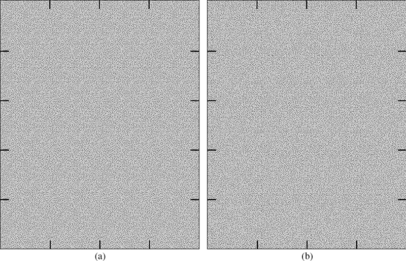
FIGURE 10.2
Illustration of the tiling artifacts created by (a) a single repeating blue-noise dither of size 108 × 108 pixels and (b) ten randomly selected dither arrays of size 108 × 108 pixels with a common border region [18].
To date, the various blue-noise dither array construction algorithms fail to fully achieve the smooth textures of error diffusion due to their reliance on steepest descent algorithms to minimize a visual cost measure, resulting in the algorithms falling into local minima. As such, this chapter introduces a postprocessing stage based on centroidal Voronoi tessellations (CVTs) to design dither arrays that, when thresholded with at a constant gray level, yield binary patterns that approximate the ideal blue-noise pattern regardless of the input gray level. This algorithm allows for a fine tuning in the distribution of minority pixels and a fine control over the quality of binary patterns at different gray levels. Centroidal Voronoi tessellations have been used in many applications ranging from data compression to optimal quadrature rules, optimal representation, quantization, clustering [15], and also halftoning. In halftoning, CVTs have been used before [16], [17] for the automatic generation of stipplings, which is a method traditionally performed by artists to represent continuous tone images as black an white images.
In Reference [17], an initial binary image, created using some halftoning algorithm is optimized through the use of weighted Voronoi digrams, using the original continuous tone image as the density function. This approach leads to good results but involves a high computational load since numerical integrations have to be performed at each iteration of the algorithm. Techniques to precalculate dot distributions, and then use look up tables to generate the halftone are also presented in Reference [17], but the quality of the halftones obtained degrades considerably with respect to the initial approach. In general the usefulness of CVTs for any application is based on its minimization properties and the capacity to create uniform distributions of dots. The algorithm presented here takes advantage of these properties to optimize the distributions of minority pixels in the binary patterns of the array. By introducing a modification of Lloyd’s algorithm, this optimization can be controlled, yielding binary patterns of even quality across the complete grayscale.
Now regardless of the construction method, the use of the dither array technique for halftoning continuous tone images have a fundamental problem related with the unavoidable tiling process of multiple copies of the dither array. As demonstrated in Figure 10.2a, the tiling creates a globally periodic halftone that is visible to the human eye. To overcome this difficulty, Reference [18] explored the possibility of constructing multiple dither arrays with component arrays tiled end-to-end in a random ordering. As shown in Figure 10.2b, this process involves constructing dither arrays with a common border, such that each pattern satisfies a wrap-around property with itself and all other component masks. However, the authors offered no criteria by which to set the size of the common border region, where too small a region leads to texture discontinuities between tiles while too large a region leads to visible tiling artifacts in the bands of the common region.
Along similar lines as described above, Reference [19] proposed the use of multiple small blue-noise screens, designed using direct binary search that could be tiled in a random order to yield high-quality halftones with an overall screen that is periodic but not having periodic artifacts. A similar approach was then offered in Reference [20] which proposed the use of screen tile indices as a watermark. Finally, Reference [21] proposed the use of multiple small constant binary texture tiles, arranged in any manner, to design highly compressible halftones.
This chapter presents a generalization of the approach first offered in Reference [18], by which the size of the common border region between component arrays is optimized as a function of the gray level. In addition, this chapter also reviews the extension of the stochastic dither arrays to nonzero screen angles, taking advantage of the human eye’s reduced sensitivity to diagonal correlation. This technique can be easily extended to color halftoning, where the possibility of tiling artifacts can be further reduced by using different screen angles for each color, as performed in traditional clustered-dot dithering.
In closing this chapter, the focus is shifted on the especially challenging problem of lenticular printing, which spatially multiplexes a series of component images to create a composite image as illustrated in Figure 10.3 [22]. These images are then transferred onto the backside of a lenticular lens array. When viewed through the lenses and depending on the incident angle through the array, the human eye sees a single de-interlaced component image. Oriented horizontally, the rotation of the lens array creates an animated image sequence. Oriented vertically, the lens array forms a stereoscopic pair that, given a sufficient number of component viewing angles, creates a full-color holographic display. Within the printing industry, lenticular imaging is most commonly associated with advertising, and in particular, most observers will associate lenticular printing with movie posters and other kiosk displays.

FIGURE 10.3
Illustration of the lenticular imaging process where: (top-center) images are divided into strips and are interlaced together into on graphic, (right) the graphic is printed directly onto the back of an extruded lens, and (bottom-right) the lenticule isolates and magnifies the interlaced image beneath, depending on the angle of observation, such that if the lenticule runs vertically, then a different image is delivered to each eye to create a 3D image. If the lenticule runs horizontal, then a rotation of the lens array creates an animation effect.
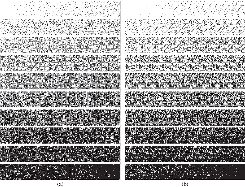
FIGURE 10.4
The halftoned grayscale ramps (a) before and (b) after downsampling using a traditional void-and-cluster dither array.
Due to the manner in which the lens array de-interlaces the component images, the use of a blue-noise dither array to halftone the composite image creates a noisy uncorrelated appearance as demonstrated in Figure 10.4. So as an attempt to maintain a smooth homogeneous distribution of printed dots in the composite image while also achieving a smooth blue-noise appearance in the component de-interlace images, this chapter introduces a modified technique for constructing blue-noise dither arrays that constrains their construction to maintain a smooth texture in both their original form as well as in their downsampled renditions. Specifically, the construction of these lenticular aware dither arrays will be studied by means of the void-and-cluster algorithm [2] where the computational complexity associated with this technique of converting a continuous tone pixel value into a binary value is a pointwise operation, requiring no additional complexity than in a traditional halftoning application.
10.3 Dither Array Construction
The masking process is a point process by which each pixel of the continuous tone input image f[n] of G gray levels is compared to a corresponding pixel in a threshold matrix S[n] of size M × N, which is called a mask or screen. If the input is greater than the threshold at position n, the binary output denoted by b[n] is set to one or otherwise to zero. In the masking processes, there is a distinct output binary pattern Ii corresponding to each constant input of gray level i with i ∈ { 0, 1,..., G − 1}. The number of pixels set to one in each binary pattern corresponds to the gray level it represents. The parameter I0 is the all zero matrix while IG−1 is the all ones matrix. And Ii has pixels set to one.
If a position in Ii0 is set to one, at gray level i0, that position remains set to one for any other Ii1 with i1 > i0. Conversely, if a position in Ii2 is set to zero, at gray level i2, then Ii1 is set to zero in the same position for any i1 < i2 (see Figure 10.5). These restrictions are called stacking constraints given by
Having all the binary patterns corresponding to each of the input gray levels, the threshold matrix S[n] is given by
and the output of the masking process is
The order in which binary patterns are designed has an important impact on its quality, since with advancing in the process more and more pixels are constrained leaving less room for the selection of new minority pixels.

FIGURE 10.5
Stacking constraints for gray levels i0< i1< i2. White pixels represent a 1, black pixels represent a 0, and gray pixels represent an undetermined value in Ii1. These values are the ones that must be set to either 1 or 0 using the binary pattern design algorithm.
In the process of designing Ii1 based on previously designed patterns Ii0 and Ii2 with i0< i1< i2, the stacking constraint implies that there would be pixels constrained to be one in Ii1 and pixels constrained to be zero, leaving
unconstrained pixels to be determined at the design stage. The criterion to select the best design order would be to maximize the number of undetermined pixels at every stage, since this allows to generate better binary patterns using the appropriate algorithm. A way to maximize Equation 10.4 is by having i2 and i0 as far as possible at every iteration and that is accomplished if the design order pivots between the extremes of the grayscale, that is, i = 0, G − 1,1, G − 2,...,(G − 2)/2. Following this ordering, the base patterns Ii0 and Ii2 always will be in opposite sides of the grayscale. The pixels considered as minority pixels are the ones set to one for Ii0 and to zero for Ii2.
As it is desirable to use the same algorithm to create binary patterns at either end of the grayscale range, regardless of the definition of a minority pixel, two sets of binary patterns defined as (assuming G even) are considered here. These binary patterns correspond to binary patterns in the mask, as for i = 0,...,(G − 2)/2 and for i = (G − 2)/2 + 1,...,G − 1. The letters b and w stand for black (bits set to zero) and white (bits set to one) since the patterns in arises for input gray levels i > (G − 1)/2 and the patterns in for i < (G − 1)/2. Using these two sets, a minority pixel will always be equal to one in any given pattern and the same algorithm can be used either to design . The design order proposed is then and the stacking constraints reformulated in terms of are
and
Once the two sets of binary patterns are designed, the mask is obtained by adding up both sets in two partial threshold matrices
and then calculating
where 1M×N is a matrix of dimension M × N filled with ones.
Each binary pattern is designed based on the previously designed binary patterns and for the case of is based on the patterns . Starting from as the all zero matrices, the algorithm that determines where to locate new minority pixels in to generate consists of a proper number of minority pixels being added to such that the resulting pattern represents gray level i (that is, has pixels set to one). If the number of pixels set to one in , then the number of pixels needed to create is Ki = Ni − Ni−1. These Ki pixels are placed one by one using the same procedure as in void-and-cluster [2]. The binary pattern is circularly convolved with a human visual system filter model B and then a new minority pixel is added in the position n* corresponding to the minimum of the filtered pattern, subject to the stacking constraint
such that
Instead of the traditional Gaussian visual model , the following model
can be used and tuned to increase the likelihood of minority pixel placement along vertical or diagonal directions (see Figure 10.6).
The parameter p determines the degree of isotropy and also influences the likelihood of minority pixel placement. By choosing values of p < 2, the likelihood of placing minority pixels in diagonal directions is increased since the L p norm has greater values than the L2 norm in diagonal directions and thus smaller values of the filter. For p > 2, the filter takes a square shape, product of the approximation of the Lp norm to the infinity norm as p grows. In this case, the likelihood of placing minority pixels along horizontal and vertical directions increases. This filter also has the particularity that along the vertical and horizontal axis it always decays as the Gaussian for any p; the setting p = 2 yields the two-dimensional Gaussian filter. Here, the values of p and the variance σ = λb are adjusted according to the gray level of the binary pattern being generated.

FIGURE 10.6
(a) Level curves of the filter with p = 1.5 and σ = 2, (b) filtered binary pattern of size 32 × 32, (c) level curves of the filter with p = 3 and σ = 2, and (d) filtered binary pattern of size 32 × 32. The * symbols denote local minimums and • symbols indicate the locations of minority pixels in the pattern.
With regards to the parameters defining the visual model, Reference [23] established that the mean distance between minority pixels in an ideal blue-noise pattern is determined by the principal wavelength
where g = i/(G − 1) is the gray level represented by the pattern and λb is the principal wavelength of the pattern. Furthermore, the same work studied the influence of the regular grid on the spectral characteristics of binary patterns and, in particular, the aliasing effects that appears at gray levels in the region 1/4< g < 3/4. From that study, it is known that to avoid disturbing artifacts and to maintain radial symmetry in the spectrum, some amount of clustering must be allowed in the region 1/4< g < 3/4 while for the region g < 1/4 and g > 3/4, the dots are mostly isolated and the principal wavelength can be used as an accurate approximation of the interpoint distance. A good method to design binary patterns according to this model is one that is capable of maintaining the interpoint distance as uniformly as possible for g < 1/4 and g > 3/4 and that also allows some clustering in the region 1/4< g < 3/4 while keeping radial symmetry.
10.4 Blue-Noise Patterns and CVTs
The algorithm proposed for constructing dither arrays in this section is a hybrid algorithm that smoothly switches the binary pattern design method between the regions g < 1/4, g > 3/4, and 1/4< g < 3/4. For the region g < 1/4 and g > 3/4, a variation of Lloyd’s algorithm is proposed to improve the uniformity of interpoint distances that can be tuned according to the gray level and that is capable of optimizing a binary pattern without significantly disturbing the previously designed binary patterns. On the other hand, for the region 1/4< g < 3/4, the criteria to design binary patterns have to be based on the minimization of the low-frequency content and the preservation of the radial symmetry of the spectrum, rather than in the homogenization of the interpoint distances. As such, any of the commonly utilized dot placement algorithms can be selected. In particular, the void-and-cluster algorithm is used since it is one with less complexity and, as will be demonstrated later, leads to very good results if used in conjunction with the Lloyd optimization stage and with a specially tuned filter.
The proposed variant of Lloyd’s algorithm, described in this section, involves iteratively tweaking the position of minority pixels within the component dither patterns using Voronoi tessellations where, in order to escape the local minima of void-and-cluster, the discrete-space dither patterns are mapped to continuous-space. The points are then mapped back to discrete-space after completing the optimization. This relaxation of discrete to continuous-space allows for a smooth and continuous optimization of the points distribution, which considerably improves the quality of the final binary pattern. As the discussion constantly goes from one space to the other, it is fundamental to clearly define the discrete and continuous spaces, introduce a proper representation of binary patterns in both spaces, and define the mappings between the two spaces.
This description begins by defining the discrete space of minority pixels as
and the continuous space of minority pixels as
where n = [m,n] are the discrete coordinates of a minority pixel and z = (x,y) are its continuous coordinates. Each binary pattern in the discrete space will be represented by an M × N binary matrix with Ni = ⌊MNi/(G−1) + 0.5⌋ entries set to one. In addition, the binary pattern are defined, that corresponds to the set of pixels swapped to one from to Ibi, according to the stacking constraint (the definition of is analogous). Each binary pattern has a number of minority pixels Ki such that Ni = Ni−1 + Ki.
Based on the definition of , any binary pattern can be expressed as
On the other hand, in the continuous space, the corresponding representation of the binary pattern is the set of Ni points such that zj = (nj,mj), where nj = [mj,nj] are the coordinates of each pixel set to one in . The set is defined as the set of points corresponding to each pixel set to one in (and analogously for . As in the discrete case, the binary patterns can be expressed as a function of the sets as follows:
Now, while the mapping to go from the discrete to the continuous space is clearly defined for each minority pixel as zj = (nj,mj), the inverse mapping is not clearly defined since the continuous space has a infinite number of possible points in it whereas discrete space contains only a finite set of elements. Therefore in any mapping, different sets of points in the continuous space will have the same discrete representation. The inverse mapping used here is the following.
Given a set of points in the continuous space , the associated matrix in the discrete space Ii is defined by quantizing the coordinates of the points zj = (xj,yj) such that
and the pixels in Ii according to
This mapping is denoted by , and as long as the points in are sufficiently separated (d(zi, zj) > 1/21/2 ∀ i, j), then this mapping returns a matrix Ii with the same number of minority pixels as the input set .
Given a set of K points that will be called here as the set of generators, the Voronoi tessellation is defined as the collection of K subsets such that each Vi is given by
Note that Vi is the set of nearest neighbors to the point zi under the distance metric d(·,·) and also that this collection of subsets covers the whole set Ω except only by the borders of the Voronoi regions. Figure 10.7a depicts an example of a Voronoi tessellation of four points in which a wrap-around Euclidean distance was used. Evidently for the same set of points there are different Voronoi tessellations, depending on the distance metric used. A thorough review can be found in Reference [24] where many variations and applications of Voronoi tessellations defined for different distances are presented. The distance used here is the Euclidean distance that wraps around the set Ω. This selection is due to the fact that Voronoi tessellations are used in the design process of binary patterns, and all binary patterns in a dither array must have the wrap-around property.
Besides the previous definitions, the definition of the centroid of a Voronoi region is also necessary. As a consequence of the distance metric used, it can be demonstrated [24] that all the Voronoi cells Vi are convex polygons. Then, denoting its vertices by vi = (xi,yi), the definition of the centroid of a Voronoi cell Vi is given by
where is the area of the cell and vi = (xi,yi) are the coordinates of its vertices.

FIGURE 10.7
(a) Example of Voronoi tessellation using the wrap-around distance, where Vi are the Voronoi cells, the centroids of the cells, and zi its generators; (b) Voronoi tessellation of a random distribution of generators (30 points); and (c) Centroidal Voronoi tessellation (30 points).
Centroidal Voronoi tessellations (CVTs) are a particular kind of Voronoi tessellations in which all the centroids of the cells corresponds to its generators zi, that is, for all i. Figures 10.7b and 10.7c show examples of a regular and a centroidal Voronoi tessellation, respectively. As it can be appreciated, the centroids and generators do not coincide, in general, for a given distribution of points. There are various method to construct CVTs [15]; Algorithm 10.1 depicts popular Lloyd’s method. In the following, a modification of this algorithm is used as a second stage of the binary pattern design, as a global optimization over the whole binary pattern constructed using the void-and-cluster algorithm.
ALGORITHM 10.1 Lloyd’s algorithm.
Set a starting distribution of points .
Calculate the Voronoi tessellation generated by the distribution.
Calculate the centroids of each Voronoi cell Vi according to Equation 10.21.
Replace the generators by the centroids .
Terminate if the maximum number of iterations is reached; otherwise do step 2.
From the binary pattern created by means of void-and-cluster, its continuous version is obtained as . The set is the continuous version of the pixels added to go from , and each set is composed of individual points denoted by zj,l. The subindex j identifies the stage in which the point was introduced, and the subindex l identifies each individual point within that stage. In the following steps, the integer constraint over the coordinates of minority pixels is relaxed and they are treated as points in the continuous space. Eventually, they have to be remapped to the discrete space, but this step is performed after the optimization of interpoint distances had converged. Before explaining the modified Lloyd’s algorithm used for the optimization of binary patterns, a set of constants μj needs to be defined; these constants are associated to each of the minority pixels which are used to control its mobility. The values of μj go from zero to one, with zero meaning that the minority pixel is not able to move at all, and one meaning complete freedom of movement.
ALGORITHM 10.2 Modified Lloyd’s algorithm.
Start with the set formed from all previous patterns.
Assign a weight μj to each point in the set of generators .
Compute the Voronoi tessellation associated with .
Calculate the centroid of each Voronoi cell in the tessellation.
Update .
Terminate if the maximum number of iterations Nmax is reached and output ; otherwise go to step 3.
Taking as input the continuous version of the binary pattern , the steps of the modified Lloyd’s algorithm are listed in Algorithm 10.2. In contrast to the traditional void-and-cluster algorithm in which once the minority pixels are located they remain unchanged for the rest of the process, this two-step algorithm of void-and-cluster followed by Lloyd’s algorithm permits the soft placement of minority pixels. It takes into account several binary patterns in which minority pixels are allowed to move with respect to their initial positions.
As an illustration of the improved spatial distribution of minority pixels afforded by Lloyd’s algorithm, Figure 10.8 depicts three different binary patterns generated using void-and-cluster (VAC) [2], direct binary search (DBS) [14], and centroidal Voronoi tessellations (CVTs). The patterns are compared in terms of their radially averaged power spectral densities (RAPSD) defined in Reference [25] by dividing the Fourier domain into a series of non-overlapping annular rings and taking the average power within each ring. The power spectra are being generated by means of Bartlett’s method of averaging periodograms. In Figure 10.8, the pattern resulting from a CVT is clearly the one with less power at low frequencies and the one that has the most isotropic distribution of points.
With regards to adding points in subsequent dither patterns under the stacking constraint, the Lloyd’s process allows for the early added points to reconfigure themselves in order to yield a more uniform distribution in the emerging binary pattern. The amount of movement allowed to previous minority pixels is controlled by the constant μj in such a way that in each iteration smaller constants are assigned to older points. By doing so, binary patterns are altered for a few design stages after their creation, but eventually converge to a fixed distribution. The drawback of the continuous optimization is that in the process, the stacking constraints with respect to the complementary set of binary patterns can be violated. To account for that, after the optimization, the output is quantized and the stacking constraints in Equation 10.6 are checked. If some of the points do not meet the stacking constraints, they are removed one by one and relocated using the same procedure as in the first stage (see Equation 10.9). The resulting pattern is converted to its continuous version and used in the next iteration to generate .
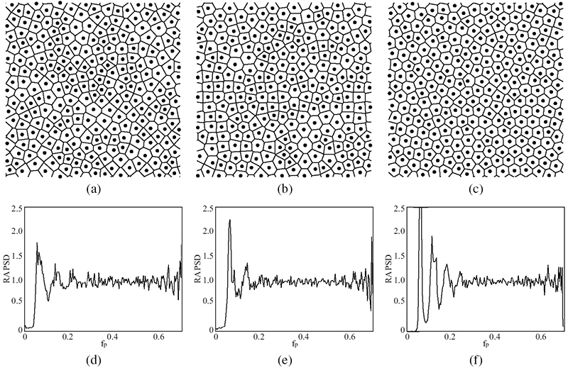
FIGURE 10.8
Centroidal Voronoi tessellations of patterns from (a) VAC, (b) DBS, and (c) CVT. Radially averaged power spectral densities (RAPSD) of patterns from (d) VAC, (e) DBS, and (f) CVT.
The set of parameters used at each component pattern change with the gray level where in the first stage of void-and-cluster, the parameters p and σ control the likelihood of minority pixel placement. In the second stage, the parameters μj and Nmax need to be set; μj parameters control the mobility of each point, and Nmax denotes the number of iterations of the modified Lloyd’s algorithm. As explained in Section 10.3, there are two different regions of the grayscale in which the criteria used to design the binary patterns change. For g < 1/4 and g > 3/4, the goal is to optimize the interpoint distances. For 1/4< g < 3/4, the goal is to reduce the low frequency content and to maintain the radial symmetry in the spectral domain. In the first stage of the design process, it was found through extensive simulation that the set of parameters giving the best results are p = 1.6 and σ = λb for g < 1/4 and g > 3/4, and p = 2 and σ = 1.5 for 1/4< g < 3/4. For g < 1/4 and g > 3/4, the process to design the mask is based on the binary pattern design algorithm presented. For 1/4< g < 3/4, the process is based on a searching process using the modified filter.
As the second stage aims to uniformly distribute the added points, more iterations of Lloyd’s algorithm must be performed for lighter and darker gray levels than for midrange gray levels. The values used for the masks shown in this chapter are Nmax = 50 for the first two binary patterns , and Nmax = 10 for the remaining patterns. The selection of the number of iterations was determined experimentally and might change for different mask sizes. The optimal value has to be determined in each case. Regarding the parameter μj, it was found that in lighter and darker regions of the grayscale bests results are obtained if only two binary patterns are optimized at a time while for midrange gray levels up to four binary patterns can be optimized. As such, the values of the constants are updated at each iteration in an exponentially decreasing sequence, initializing all the constants at μj = 0.94, and then updating their values as for g < 1/32 and g > 31/32, and for 1/32< g < 1/4 and 3/4 < g < 31/32. For 1/4 < g < 3/4, the parameter μj is set to zero since no Lloyd optimization is performed.
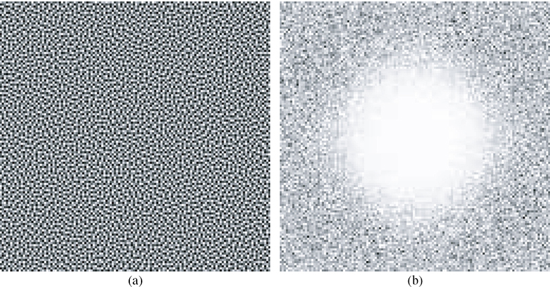
FIGURE 10.9
The resulting eight-bit 128 × 128 blue-noise dither array in (a) the spatial domain and (b) the spectral domain.
The mask design process starts by setting , and then the binary patterns up to are designed using the two-step procedure of void-and-cluster followed by Lloyd’s algorithm under that stacking constraint. For subsequent patterns in the range from i = (G − 2)/4 +1 to i = (G − 2)/2, a searching process is used where, given , the pattern is designed by adding Ki minority pixels to to complete the Ni = ⌊MNi/(G − 1) + 0.5⌋ necessary for gray level i. The minority pixels are added one by one, subject to the stacking constraints in Equations 10.5 and 10.6 in positions n* given by
Analogously, is designed adding Ki minority pixels to in positions n* given by
The process continues until the two last binary patterns are generated.
It is important to note that only the continuous versions of the binary patterns are stored, updating the sets at each iteration. In contrast to the algorithm used for i < (G − 2)/4, there is no optimization of the interpoint distance through Lloyd’s algorithm, and the placement of minority pixels is always performed in the discrete space in the range i = (G − 2)/4 + 1 to i = (G − 2)/2. However, their continuous space versions are stored to reconstruct the discrete patterns at the end according to Equation 10.24. The matrices B and W are built according to Equation 10.7 and the mask is generated according to Equation 10.8, where the sets of binary patterns in the discrete space are recovered from their continuous versions by computing
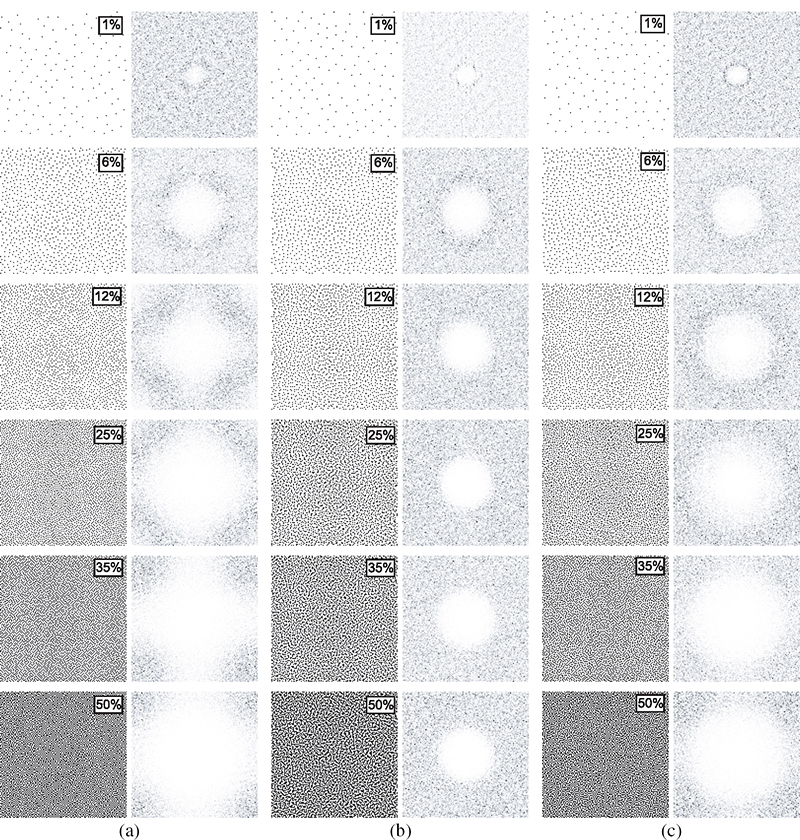
FIGURE 10.10
Comparison of binary patterns generated using (a) VAC, (b) DBS, and (c) CVT algorithm. The number shown over the binary patterns is the ink coverage percentage of the pattern and the column on the right of each binary pattern correspond to the absolute value of its DFT with the DC component removed.
Figure 10.9 depicts the resulting dither array along with the magnitude of its Fourier transform, created using this process. As expected, this array has a highpass power spectrum.
In order to compare the quality of binary patterns from masks designed using the Voronoi optimization algorithm, Figure 10.10 depicts a set of binary patterns from VAC, DBS, and CVT masks along with their Fourier transforms. These patterns correspond to only half of the grayscale, since as a consequence of the design order used, the characteristics of patterns in diametrically opposed gray levels are almost equal.
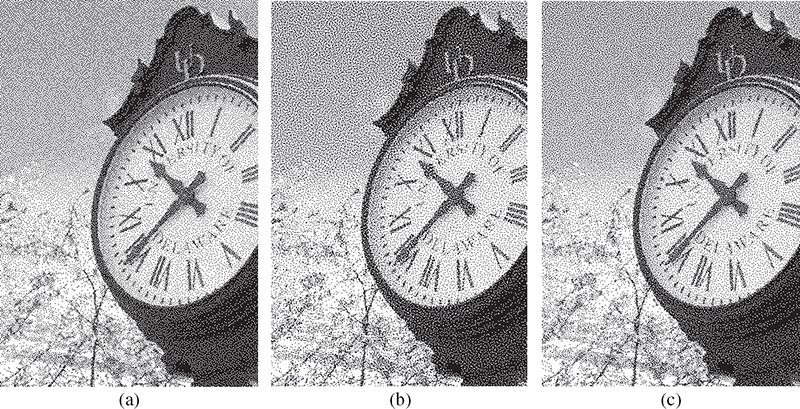
FIGURE 10.11
Halftoned images resulting from the masking process using (a) VAC mask, (b) DBS mask, and (c) Voronoi optimized mask. The size of the rendered image is 400 × 602 pixels and it is printed at 160 dpi.
The binary patterns from the VAC mask (Figure 10.10a), designed using the VAC algorithm [2] with a fixed variance of the filter set to σ = 2.5, have much of their power in the high-frequency region, with power accumulation in diagonal directions for g = 1/2. As noted in Section 10.4, a good blue-noise mask must have some degree of clustering for 1/4 < g < 3/4; the VAC mask does not present any clustering in that region, yielding a noisy appearance and the emergence of artifacts at midrange gray levels. The patterns from the DBS mask (Figure 10.10b), on the contrary, have a more stable appearance and a much more symmetric spectrum, but at the expense of a higher degree of clustering for 1/8 < g < 7/8 with power accumulation at lower frequencies. Finally, the patterns from the CVT mask (Figure 10.10c) are in between the patterns from VAC and DBS, having less low-frequency content than DBS patterns, but at the same time preserving the radial symmetry in the frequency domain for all gray levels. This is understandable because the Voronoi optimization algorithm can be tuned to smoothly switch the criteria for binary pattern design in different regions of the grayscale. Through the appropriate selection of parameters, one can design patterns that are better approximations to the ideal blue-noise pattern. Figure 10.11 presents halftoned images using the VAC, DBS, and CVT masks.
10.5 Artifact-Free Dither Arrays
As shown in Figure 10.2, the problem with halftoning by means of a single, blue-noise dither array is that, through the process of tiling, the resulting halftone becomes periodic and at high print resolutions, this periodicity imparts a visually disturbing texture onto the image. Reference [18] addresses this problem by generating a set of unique dither patterns such that, regardless of their ordering, would show no apparent discontinuities in texture when tiled together. This phenomenon is here referred to as a wrap-across property. The resulting halftoning process would reduce the tiling artifacts of traditional dither array halftoning while maintaining the computational simplicity of a point-process.
In order to generate a set of dither arrays that satisfy the wrap-across property, the method of Reference [18] starts from a dither array generated according to the traditional technique. From this initial array, the method generates a set of subsequent dither arrays, where the boundary pixels are constrained to correspond exactly with those of the initial array. Specifically in this chapter, the initial sets of binary patterns are generated for the first dither array S1 using the algorithm described in previous sections. Given this initial array, a mask M is defined as a binary image with the same row and column dimensions as the proposed component binary patterns. This matrix has the boundary pixels of k rows at the top and bottom and k columns at the right and left equal to one, indicating that these pixels must remain unchanged in the new dither array. The center pixels of M are set to zero, indicating that these pixels need to be designed independently.
Having the mask M, the process begins by generating the set of binary patterns corresponding to the second mask S2. Starting from as all zero matrices, the pattern is generated by adding K1 = ⌊MN1/(G − 1) + 0.5⌋ ones to . The term is initialized as and the remaining ones are added as follows:
For M[n] = 0, the remaining minority pixels to complete the K1 pixels are added one by one in positions n*, where
In the next step, the continuous space version of the resulting pattern from the previous process is optimized using the modified Lloyd’s algorithm with the constants μj set to zero for the pixels in the common border and to one for the rest of the pixels. The term is obtained by mapping the result of the optimization to the discrete space as .
The second binary pattern is generated in a similar way. First, the pattern is initialized as and the pixels in the common border are set as in positions where M[n] = 1. The remaining pixels are added in positions n*, where
Then, the continuous version of is optimized setting the constants μj to zero for pixels in the common border and to one for the rest. The discrete version of the binary pattern is obtained by doing . If for some pixels the conditions in Equations 10.5 and 10.6 are not met, these pixels are removed one by one and placed according to Equation 10.27. For the first two binary patterns, the number of iterations of Lloyd is set to Nmax = 50. For the remaining patterns, the parameters are set as described previously. The remaining binary patterns {: i = 2,3,...,(G − 2)/2} are designed in an analogous way as in Section 10.4 with the difference that at each iteration the binary patterns are generated by first copying the common border pixels and in positions where M[n] = 1. The remaining pixels to complete the Ki necessary are added in positions where M[n] = 0 according to Equations 10.22 and 10.23 and optimized in the same way as the first two patterns . The results of applying this algorithm to the dither array presented in Figure 10.9 are shown in Figure 10.12 with clear blue-noise characteristics.
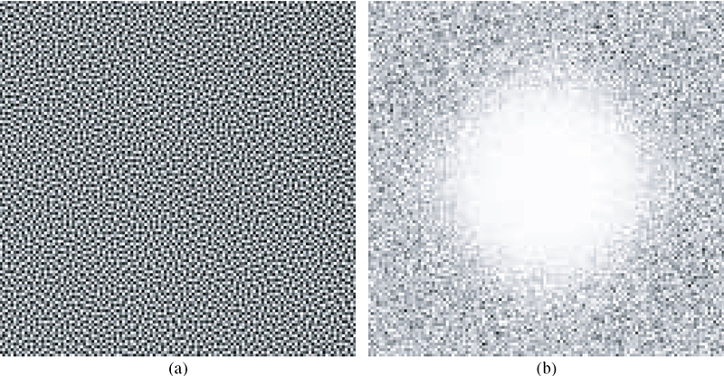
FIGURE 10.12
The resulting eight-bit 128 × 128 complementary blue-noise dither array derived from dither array of Figure 10.9 in (a) the spatial domain and (b) the spectral domain.
In order to further minimize the likelihood of visible tiling artifacts deriving from the common boundary region, the goal should be to reduce k, which denotes the number of pixels, by defining the width of the boundaries in M. This approach is limited by the expected spacing between printed dots of the component dither patterns such that too small k results in discontinuities in texture near the boundary between two unique dither patterns. Here, k = ⌈λb⌉ is defined as a gray-level dependent variable equal to the principal wavelength, defined in Equation 10.12. This way takes advantage of what is known from Reference [10] about the correlation between printed dots of blue-noise patterns, ensuring that unconstrained thresholds of one component array are twice λb apart from those of neighboring component arrays. Figure 10.13a shows the result of applying the adaptive border technique and Figure 10.13b shows the common pixels between two complementary dither arrays resulting from the approach of Reference [18]. The common pixels near the boundaries are greatly reduced for the adaptive technique, leading to a reduction in tiling artifacts as well. Figure 10.14 depicts the corresponding halftone pattern representing the 70% gray level using ten randomly selected masks with adaptive common border.
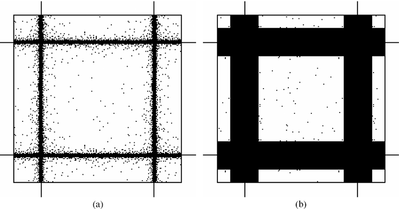
FIGURE 10.13
The common pixels, marked in black, between the complementary dither arrays: (a) the result of adapting the common border according to λb, (b) the result of setting a common border to ten pixels.
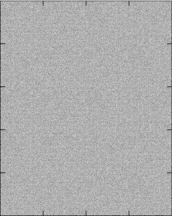
FIGURE 10.14
Illustration of the tiling artifacts created by ten randomly selected dither arrays with a minimized common border region.
As a further means of reducing the visibility of the repeating boundaries, one can rely on the human visual system’s reduced sensitivity to diagonal correlation and generate dither arrays at rational screen angles. In particular, it is known that, at rational screen angles, the halftone cells of a traditional amplitude modulation screen form a regular tiling pattern. Combining these halftone cells (on the order of 12 × 12 or 16 × 16 pixels) into larger cells allows creating a regular tiling pattern whose cell period is on the order of a traditional blue-noise dither array (128 × 128 or 256 × 256). Figure 10.15 illustrates the tiling pattern created by such an arrangement using a 27° screen angle with a minimized border region and cell size of 128 × 128. Now, because the dither array can be aligned at any rational screen angle, an obvious extension of the proposed dither array scheme is to vary the screen angles between color primaries as is performed with traditional, clustered-dot ordered dithering. By doing so, the likelihood of tiling artifacts is further minimized, as could also be achieved by varying the size of the component dither arrays between colors. This is especially advantageous for small screen sizes, where the common border region accounts for a significant percentage of dither array area and hence, a large portion of the final halftone contains a repeating artifact.
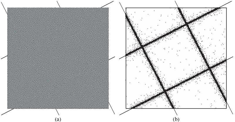
FIGURE 10.15
(a) The result of tiling nine dither arrays created with the adaptive border technique at an angle of 27°, and (b) common pixels, marked in black, between the base dither array and nine common border dither arrays.
To study the reduction in tiling artifacts achieved by the adaptive common border technique presented in Section 10.5, two patches of 3 × 3 dither arrays are compared. The first one denoted by Y corresponds to the tiling of nine randomly selected arrays generated with the adaptive technique, and the second one denoted by W correspond to the periodic tiling of one dither array S1. Denoting by Si the common border dither arrays, the cells Y and W are given by
To quantify the amount of reduction in tiling artifact, the autocorrelations of both cells Y and W are evaluated and the peaks present at multiples of the dither array size are compared. Calling FY = FFT(Y) and FW = FFT(W), where FFT stands for the fast Fourier transform, the autocorrelations can be obtained as RYY = IFFT(|FY|2) and RWW = IFFT(|FW|2), with the DC component of FY and FW subtracted before calculating the inverse FFT (IFFT). Figure 10.16 shows the values of both autocorrelations evaluated at the horizontal axis [0,k], since it is along horizontal and vertical directions where the peaks in the autocorrelation are found. It can be seen that the peaks at k = 128 and k = − 128 are significatively reduced in the cell containing the adaptive border arrays with respect to the periodic cell.
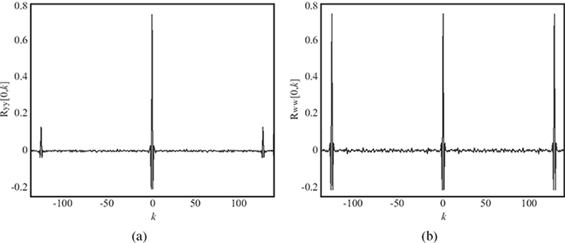
FIGURE 10.16
(a) Autocorrelation of Y evaluated at [0,k]. (b) Autocorrelation of W evaluated at [0,k]. The size of the dither arrays used were 128 × 128 pixels.

FIGURE 10.17
Gaussian lowpass filters used by VAC: (a) standard and (b) lenticular aware filter. Darker colors indicate larger filter values.
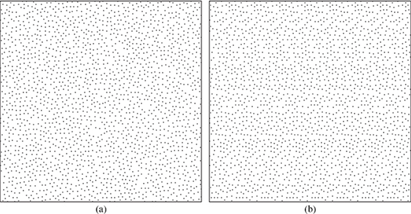
FIGURE 10.18
(a) The lenticular aware dither pattern. (b) The corresponding dither pattern constructed by repeating a down-sampled rendition eight times.
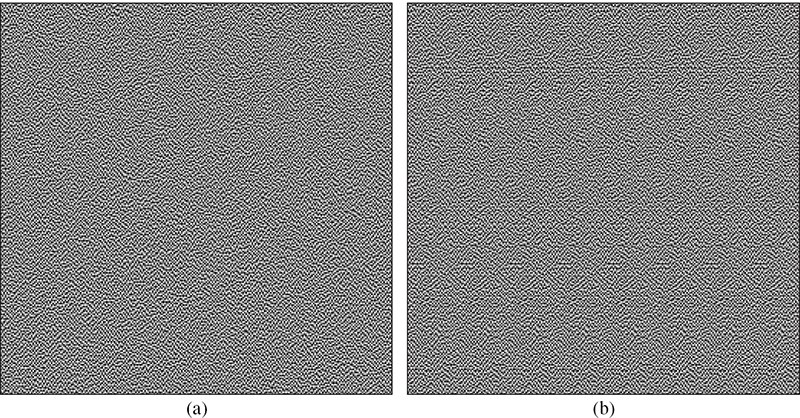
FIGURE 10.19
(a) The lenticular aware dither array. (b) The corresponding dither array constructed by repeating a downsampled rendition eight times.
10.6 Lenticular Screening
Now, in order to modify the void-and-cluster algorithm to produce lenticular aware dither arrays, the lowpass filter is modified to maintain smooth textures in the downsampled image such that

FIGURE 10.20
(a) The magnitude of the Fourier transform of the lenticular aware dither array. (b) The red-noise voids, indicated by white ovals, caused by the upsampling operation on the lowpass filters used by VAC.
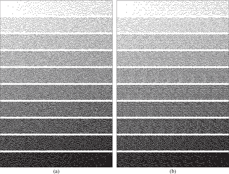
FIGURE 10.21
The halftoned grayscale ramps (a) before and (b) after downsampling using a lenticular aware dither array.
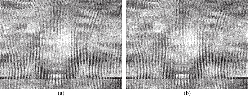
FIGURE 10.22
A composite lenticular image halftoned by means of (a) a traditional VAC dither array and (b) a lenticular aware VAC dither array.
where N is the number of printed pixel columns under each lens of the lenticular image. In the case of having eight pixel columns under each lens, Figure 10.17 compares the new lenticular aware filter against a traditional VAC version. Applying this new filter, Figure 10.18 shows the dither pattern before and after downsampling, where no discontinuity in texture can be observed, although there are some unwanted hole artifacts. As for the resulting dither array, Figure 10.19 shows the final dither array and the corresponding dither array formed by first downsampling the original array by a factor of eight and then tiling the resulting array eight times to create a new 256 ×256 array. Figure 10.20a presents the magnitude of the raw dither array’s Fourier transform that shows the effects of the upsampling operation on the lowpass filter. This results in multiple red-noise voids, which are indicated in Figure 10.20b by the white ovals superimposed over the Fourier transform plot.
Looking now at the dot patterns produced by this array, Figure 10.21 shows the corresponding grayscale ramp and image produced by thresholding with the lenticular aware dither array with neither dot pattern showing any significant discontinuity in texture except at extreme gray levels. To evaluate the effects of the new dither array on lenticular images, Figure 10.22 shows the halftones produced by a traditional and the new lenticular aware dither array for a lenticular image composed of eight component images with each image corresponding to single pixel-wide slices. In the composite images, neither halftone shows any discontinuity in texture caused by the dither array. However, in Figure 10.23, which shows one of the eight de-interlaced component images, one can see what looks like a white-noise halftone produced by the traditional dither array while the lenticular aware array creates a traditional blue-noise texture.
With regards to the change in texture across two neighboring component images, such as would be visible when progressing through an animated sequence, one can look at the textures produced when the composite image is downsampled by a factor one-off from its true rate, in this case downsampled by seven instead of eight. The resulting textures are visible in Figure 10.24 where, again, the traditional dither array produces a white-noise texture while the new array maintains a much smoother texture. The vertical blind effect, visible in these two figures, are a result of the transition from the eight component image back to the first component image occurring at every eight sample, since one component image is shifted with each downsampled pixel. What these two figures suggest is that as a human subject’s eye animates through the lenticular sequence, it will see larger amounts of twinkling in the traditional halftone versus the lenticular aware technique.
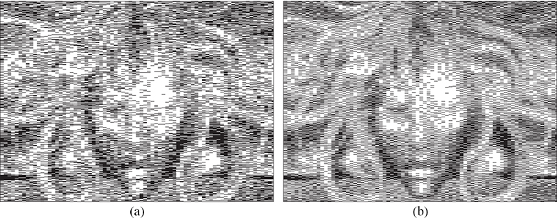
FIGURE 10.23
A de-interlaced lenticular image halftoned by means of (a) a traditional VAC dither array and (b) a lenticular aware VAC dither array.

FIGURE 10.24
A de-interlaced lenticular image downsampled by a factor of seven (one-off from the true rate of eight) and halftoned by means of (a) a traditional VAC dither array and (b) a lenticular aware VAC dither array.
A further implication of Figure 10.24 is that it suggests that the size of the lenticular aware dither array does not need to be an integer multiple of the downsampling rate, and that one could make the dither array of size KN − 1, where K is some positive integer. Such a dither array would have the advantage of producing a periodic texture in the de-interlaced image with a horizontal period of (KN)2 lenses instead of K lenses. It would still have a vertical period of approximately KN pixels, but at the printer’s native resolution, not the lens resolution. Of course, it is possible to construct non-square dither arrays with large vertical periods. The important feature here is that one can achieve much larger horizontal periods in the de-interlaced images with modest periods in the composite image. Figure 10.25 demonstrates the reduction in tiling artifacts achieved through this process, where Figure 10.25b shows the grayscale ramp produced by a downsampled rendition of the lenticular aware dither array. In summary, the lenticular aware VAC process produces consistent halftone textures in both the composite and de-interlaced renditions of a lenticular image with reduced tiling artifacts achieved by using a non-integer multiple of the downsampling rate for the dither array width. Tiling artifacts in the composite image are of no significant consequence.
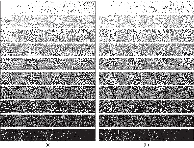
FIGURE 10.25
The halftoned grayscale ramps (a) before and (b) after downsampling using a lenticular aware dither array of size 255 × 255 pixels.
10.7 Conclusion
By introducing a concise description of the ideal spectral shape of visually pleasing dither patterns, Reference [12] introduced a means by which dither patterns could be quantitatively evaluated, and hence, one could compare multiple halftoning algorithms with the better technique being the one with a spectral profile closest in shape to this ideal model. While this cost played a fundamental role in the optimization of error-diffusion [26], [27], [28], [29], its most significant contribution may be its leading to the construction of aperiodic dispersed-dot dither arrays. While sharing many similarities to periodic clustered-dot dithering arrays, blue-noise arrays have, so far, failed to achieve the same level of variability/flexibility with their only significant variation being the dither array size.
This chapter has attempted to bridge the gap between blue-noise dither arrays and traditional ordered dithering, offering a wider range of parameters by which the user can optimize threshold placement. Through the selection of different sets of parameters μj, Nmax, p, and σ for each gray level, the textures and radial symmetry of the binary patterns obtained can be controlled with greater versatility. The amount of power accumulated along vertical or diagonal directions can be controlled by choosing p > 2 or p < 2 in the searching filter and the uniformity of the whole pattern regulated by performing more iterations of the modified Lloyd’s algorithm. In addition, an even quality across the whole grayscale can be achieved by optimizing multiple binary patterns simultaneously at each iteration, choosing the rate at which the μj constants change with each iteration.
The reduction in tiling artifacts achieved by optimizing the common border of dither arrays has proved to be significant, as shown in Figure 10.16. The design of dither arrays at rational screen angles have further reduced the presence of artifacts allowing to produce nearly artifact-free screens. Beyond the reduction in tiling artifacts, the technique of tiling common border dither arrays creates new opportunities for data encryption and digital watermarking [19], [30], [31], in which a message can be encoded in the ordering chosen for the tiling of small binary patterns.
Looking at lenticular printing, it should be noted that even simply modifications to existing techniques can produce dramatic improvements over applying traditional halftoning algorithms. This chapter has presented such a modification by altering the lowpass filter of void-and-cluster algorithm. In doing so, the proposed dither array produces smooth, blue-noise textures in both the raw composite image as well as the de-interlaced component images. Beyond this improvement, this chapter has also introduced a novel means of evaluating halftone texture in lenticular images by looking at the halftone produced by downsample one-off from the true de-interlacing rate. This new means of texture evaluation attempts to analyze the change in dot patterns across neighboring component images as would be seen in an animated lenticular sequence.
Acknowledgment
Figure 10.9 is image courtesy of the University of Delaware.
References
[1] B. Bayer, “An optimum method for two level rendition of continuous-tone pictures,” in Proceedings of the IEEE International Conference on Communications, Seattle, WA, USA, June 1973, pp. 11–15.
[2] R.A. Ulichney, “The void-and-cluster method for dither array generation,” Proceedings of SPIE, vol. 1913, pp. 332–343, February 1993.
[3] J. Sullivan and L. Ray, “Digital halftoning with correlated minimum visual modulation patterns,” U.S. Patent 5 214 517, May 1993.
[4] J. Sullivan, L. Ray, and R. Miller, “Design of minimum visual modulation halftone patterns,” IEEE Transactions on Systems, Man and Cybernetics, vol. 21, no. 1, pp. 33–38, January 1991.
[5] T. Mitsa and K.J. Parker, “Digital halftoning technique using a blue noise mask,” Journal of the Optical Society of America, vol. 9, no. 11, pp. 1920–1929, August 1992.
[6] M. Yao and K.J. Parker, “Modified approach to the construction of a blue noise mask,” Journal of Electronic Imaging, vol. 3, no. 1, pp. 92–97, January 1994.
[7] J. Allebach and Q. Lin, “FM screen design using the DBS algorithm,” in Proceedings of the IEEE International Conference on Image Processing, Lausanne, Switzerland, September 1996, pp. 549–552.
[8] B.E. Cooper, T.A. Knight, and S.T. Love, “Method for halftoning using stochastic dithering with minimum density variance,” U.S. Patent 5 696 602, December 1997.
[9] K.E. Spaulding, R.L. Miller, and J. Schildkraut, “Methods for generating blue-noise dither matrices for digital halftoning,” Journal of Electronic Imaging, vol. 6, no. 2, pp. 208–230, April 1997.
[10] D.L. Lau, G.R. Arce, and N.C. Gallagher, “Green-noise digital halftoning,” Proceedings of the IEEE, vol. 86, no. 12, pp. 2424–2444, December 1998.
[11] R.W. Floyd and L. Steinberg, “An adaptive algorithm for spatial gray-scale,” Proceedings of the Society of Information Display, vol. 17, no. 2, pp. 75–78, 1976.
[12] R.A. Ulichney, “Dithering with blue noise,” Proceedings of the IEEE, vol. 76, no. 1, pp. 56–79, January 1988.
[13] R.L. Stevenson and G.R. Arce, “Binary display of hexagonally sampled continuous-tone images,” Journal of the Optical Society of America, vol. 2, no. 7, pp. 1009–1013, July 1985.
[14] M. Analoui and J.P. Allebach, “Model based halftoning using direct binary search,” Proceedings of SPIE, vol. 1666, pp. 96–108, August 1992.
[15] V.F.Q. Du and M. Gunzburger, “Centroidal Voronoi tessellations: Applications and algorithms,” SIAM Review, vol. 41, no. 4, pp. 637–676, April 1999.
[16] O. Deussen, S. Hiller, C.V. Overveld, and T. Strothotte, “Floating points: A method for computing stipple drawings,” Computer Graphics Forum, vol. 19, no. 3, pp. 41–50, March 2000.
[17] A. Secord, “Weighted Voronoi stippling,” in Proceedings of the 2nd International Symposium on Non-Photorealistic Animation and Rendering, Annecy, France, June 2002, pp. 37–43.
[18] B.W. Kolpatzik and J.E. Thornton, “Image rendering system and method for generating stochastic threshold arrays for use therewith,” U.S. Patent 5 745 660, April 1998.
[19] D. Kacker and J.P. Allebach, “Aperiodic micro-screen design using DBS and training,” Proceedings of SPIE, vol. 3300, pp. 386–397, January 1998.
[20] Z. Baharav and D. Shaked, “Watermarking of dither halftone images,” Proceedings of SPIE, vol. 3657, pp. 307–316, January 1999.
[21] S. Kim and J.P. Allebach, “High quality, low complexity halftoning with good compressibility,” in Proceedings of the IEEE International Conference on Image Processing, Rochester, NY, USA, September 2002, vol. 1, pp. 453–456.
[22] D.L. Lau and T. Smith, “Model-based error-diffusion for high-fidelity lenticular screening,” Optics Express, vol. 14, no. 8, pp. 3214–3224, April 2006.
[23] D.L. Lau and R. Ulichney, “Blue-noise halftoning for hexagonal grids,” IEEE Transactions on Image Processing, vol. 15, no. 5, pp. 1270–1284, May 2005.
[24] K.S.A. Okabe, B. Boots, and S.N. Chiu, Spatial Tessellations: Concepts and Applications of Voronoi Diagrams. Chichester, UK: John Wiley & Sons Ltd, 2nd edition, 2000.
[25] D.L. Lau and G.R. Arce, Modern Digital Halftoning. New York, USA: Marcel Dekker, 2001.
[26] R. Eschbach and K.T. Knox, “Error-diffusion algorithm with edge enhancement,” Journal of the Optical Society of America, vol. 8, no. 12, pp. 1844–1850, December 1991.
[27] B.W. Kolpatzik and C.A. Bouman, “Optimized error diffusion for image display,” Journal of Electronic Imaging, vol. 1, no. 3, pp. 277–292, July 1992.
[28] T. Zeggle and O. Bryngdahl, “Halftoning with error-diffusion on an image-adaptive raster,” Journal of Electronic Imaging, vol. 3, no. 3, pp. 288–294, July 1994.
[29] T.D. Kite, B.L. Evans, A.C. Bovik, and T.L. Sculley, “Digital halftoning as 2-D delta-sigma modulation,” in Proceedings of the IEEE International Conference on Image Processing, Santa Barbara, CA, USA, October 1997, vol. 1, pp. 799–802.
[30] M.S. Fu and O.C. Au, “Data hiding watermarking for halftone images,” IEEE Transactions on Image Processing, vol. 11, no. 4, pp. 477–484, April 2002.
[31] Z. Zhou, G.R. Arce, and G.D. Crescenzo, “Halftone visual cryptography,” IEEE Transactions on Image Processing, vol. 15, no. 8, pp. 2441–2453, August 2003.