13 Perceptually Driven Video Shot Characterization

Analyzing a video shot requires identifying the meaningful components that influence the semantics of the scene through their behavioral and perceptual attributes. This chapter describes an unsupervised approach to identify meaningful components in the scene using perceptual grouping and perceptual prominence principles. The perceptual grouping approach is unique in the sense that it makes use of an organizational model that encapsulates the criteria that govern the grouping process. The proposed grouping criteria rely on spatiotemporal consistency exhibited by emergent clusters of grouping primitives. The principle of perceptual prominence models the cognitive saliency of the subjects. Prominence is interpreted by formulating an appropriate model based on attributes which commonly influence human judgment about prominent subjects. The video shot is categorized based on the observations pertaining to the mise-en-scène aspects of the depicted content.

Perceptual organization is the process of identifying inherent organizations in visual primitives. Simpler primitives can be organized to obtain higher-level meaningful structures. In order to group simpler primitives one needs to formulate a grouping model that specifies the grouping criteria that influence the formation of meaningful (perceptual) clusters. For example, a model of a human being can be specified as a spatial organization of parts, such as torso, head, legs, hands, and so on. Being able to detect the parts and their requisite spatial organization reinforces the belief that the human being is present in the scene. For a general video the grouping primitives need to be simple enough to be extracted from all types of objects. Further, the organization model should make use of general grouping criteria and be flexible enough to incorporate grouping evidences from an object category-specific grouping model, if available. One also needs unsupervised algorithmic procedures that can make use of the grouping model to identify salient clusters.

The principle of perceptual prominence [1] is motivated from film grammar that states that scene understanding depends on the characteristics of the scene components. Human attention gets focused on the most over-riding or prominent components in the scene. A film-maker or a painter uses the arrangement of the mise-en-scène [2] to direct visual attention across the visualization space (a scene in space and time). Perceptual prominence captures the cognitive aspects of attention, which deals with perceiving the perceptible (visual) attributes in the context of prior knowledge or expectation from the scene, and is used to identify the perceived prominent subjects. The semantics of a scene are closely linked with the way humans interpret the scene and thereby establish the visual attributes and behavioral patterns of the prominent subjects. The perceptual attribute specifications are parametrized into different prominent models that correspond to different interpretations of prominence. The behavioral aspects of prominent subjects and the mise-en-scène features are used to generate a taxonomy of interpretation of the video scene.

Many classical perceptual organization studies, which have addressed organizing and grouping primitives in images, have been recently extended to organizing primitives in the spatiotemporal domain of video. Given a pair of frames, the organization principle of smoothness (or continuity) has been used for computing optical flow, organizing moving points for planar motion [3], and estimating the dense motion field in a tensor voting framework [4]. Organization of motion fields to detect patterns, such as saddles, sinks, and sources, has been used to study qualitative behaviors of objects [5], [6]. Perceptual organization has been applied to primitives that exist over extended sequence of frames in different applications like grouping feature trajectories [7], tracking structures [8], and object extraction [9].

Attempts to quantify the saliency of organizational structures have made use of different properties like transformational invariance [10], structural information [11], local characteristics [12], and probability of occurrence of the structure [13]. There has been work on modeling pre-attentive vision [14] and computation of visual saliency [15]. Reference [16], has used perceptual features of the groupings and computed qualitatively significant perceptual groupings by repeated applications of rules. The “interestingness” of a structure is evaluated by considering its size, contrast, extent, type of similarity, and the number of groupings the structure is associated with.

This chapter presents a perceptual grouping scheme for the spatiotemporal domain of video. The proposed grouping model is motivated from the Gestalt law of common fate that states that the entities having a coherent behavior in time are likely to be parts of the same organization. The researchers in the Gestalt school of psychophysics [17], [18], [19] have identified certain relationships, such as continuation of boundaries, proximity, adjacency [20], enclosures, and similarity of shape, size, intensity, and directionality, which play the key role in the formation of “good” structures in the spatial domain. These associations have been used to identify salient groupings of visual patterns (primitive entities) in a two-dimensional visual domain [21]. However, in the spatiotemporal domain, the spatially salient grouping must show coherence (common fate) in the temporal domain. Therefore, this chapter also presents formulations for association measures which characterize temporal coherence between primitives to group them into salient spatiotemporal clusters, termed as perceptual clusters. The foreground perceptual clusters identified by the proposed perceptual grouping algorithm correspond to the subjects in the scene.

Semantic information from a video is extracted here in the form of a collection of concepts interpreted by analyzing the behavior and properties of the identified meaningful components. In order to do so, video shots are categorized into two broad categories:

Subject-centric scenes, which have one or few prominent subjects and are more suitable for object-centric descriptions that facilitate an object-oriented search [22], [23].
Frame-centric scenes, which have many subjects, but none of them can be attributed a high prominence. Hence, the overall activity depicted in the scene is the subject of interest. Such scenes can be described in terms of features and semantic constructs that do not directly pertain to the objects but characterize the gross expressiveness of the medium at the frame level or the shot level, for example, features like color histogram, dynamicity [24], tempo [25], dialogue [26], etc.

Note that the annotations for a given video scene would be more efficacious when they align with the viewer’s perception of the content depicted in the scene. Therefore, perceptual grouping and prominence principles are employed here toward the end goal of automatic semantic annotation of videos into general categories. Content specific semantic metadata can facilitate effective utilization of video information in various applications, such as transcoding, browsing, navigation, and querying.

This chapter is organized as follows. Section 13.2 gives an overview of proposed clustering methodology to extract space-time blob tracks, which are the visual primitives for grouping. Extraction of meaningful components in a video is done by applying perceptual organization principles on visual primitives. Section 13.3 describes the basic ideas behind spatiotemporal grouping and outlines the formulations of association measures that play a key role in formation of salient groupings. Section 13.4 describes the proposed spatiotemporal grouping model which is then used in a perceptual grouping algorithm to identify the foreground subjects in the video shot. Section 13.5 reports results obtained by applying the perceptual grouping algorithm to video scenes. Section 13.6 provides a general framework to evaluate perceptual prominence of the identified subjects by making use of perceptual attributes such as life span and movement, and mise-en-scène features like placement in the scene, and color contrast. The attribute specifications are parametrized into different prominence models that signify different interpretations of prominence. A taxonomy of interpretation of video scenes based on the behavior of prominent subjects is also generated. Video shot interpretation into generic categories follows from the analysis of prominent subjects in the scene. Section 13.7 uses domain knowledge in the form of learned object-part models to perform object recognition through a grouping process. This chapter concludes with Section 13.8.

13.2 Space-Time Blob Tracks

The grouping primitives are identified here as space-time regions, homogeneous in color using unsupervised clustering techniques, and modeled as tracks of two-dimensional blobs along time. Video data are multidimensional; they can be represented using two spatial coordinates (x, y), three color components (for example, RGB or LUV), and one time dimension. This makes a heterogeneous feature vector because color, space, and time have different semantics. Clustering such a six-dimensional feature space can result in undesirable smoothing across features of different semantics. Pixels having similar color but actually lying on different objects may become part of the same cluster. This leads to a higher variance along certain dimensions, which may be semantically unacceptable because the cluster is encompassing patches that belong to different objects. To ensure that the clusters model patches that are homogeneous in color and belong to the same object, one can apply clustering in stages and consider a subspace of semantically homogeneous features at each stage. Each cluster is divided into further subclusters at the subsequent level, resulting in a hierarchical clustering tree called the decoupled semantics clustering tree (DSCT) [27]. The clustering methodology and the feature subspace can be chosen as different for each level. The choice is guided by the distribution of feature points in the feature space used for partitioning the cluster.

The root node (level 0) of the clustering tree represents all the feature points, that is, pixels, in the video shot. At level 1 of the clustering tree, the entire set of pixels is partitioned along time to form video stacks or subclusters, each comprising ten consecutive video frames. Making such video stacks or sets of consecutive frames reduces the amount of data handled by the clustering algorithm at the next level. At level 2, pixels in the video stack are decomposed into regions homogeneous in color. This is done by applying hierarchical mean shift [28] to obtain clusters in the color subspace, such as the LUV color space. Hierarchical mean shift results in a dendrogram of color modes. A set of color modes are chosen as the color model. Each color cluster comprises the set of pixels that had converged to the mode during the mean shift process. At level 3, the pixels in the color cluster are partitioned along time by projecting them onto the individual frames. The clusters at this level comprise pixels having similar color and belonging to the same frame. Pixels in clusters at level 3 are modeled as two-dimensional Gaussians (blobs) using Gaussian mixture model clustering. These blobs are then tracked across successive frames to obtain blob tracks that model space-time regions. These space-time blobs are the primitive patterns to be grouped to identify the perceptual clusters, as discussed in the next section.

13.3 Perceptual Grouping in Spatiotemporal Domain

The perceptual units that serve as input to the proposed perceptual grouping algorithm are the spatiotemporal blob tracks that model regions homogeneous in color. The goal is to identify meaningful groupings of these blob tracks to form perceptual clusters.

Consider a set of patterns S = {p₁, p₂,...p_n} and a set c_k such that c_k ⊆ S. Let G(c_k) denote a spatial grouping of the patterns in c_k. The set of attributes for all the member patterns in c_k at time t are denoted as $c_{k}^{t}$ and the attributes of the complete spatial grouping considered as a single entity are denoted by G^t(c_k). A set c_k ∈ S is a perceptual cluster in the spatiotemporal domain if ${c_{k}^{t}, G^{t} (c_{k})}$ obeys a spatiotemporal grouping model that defines a salient temporally coherent organization. This model specifies a set of temporal behavior attributes for the cluster c_k and an operational method that uses these attributes to compute a grouping saliency measure for c_k. Temporal behavior attributes, for example, related to visual characteristics or contextual behavior, can be formulated for the overall grouping and the individual patterns. The proposed definition requires that in addition to the overall grouping G^t(c_k), the individual patterns in the grouping must show temporal consistency in terms of their attributes $c_{k}^{t}$ , which could be, for example, visual characteristics or contextual behavior. Such a formalism allows enforcement of specific visual and temporal behavior characteristics on some or all patterns of a grouping.

Following the proposed definition of a perceptual cluster, there are three possible types of attributes that can be used to characterize spatiotemporal saliency:

Properties of the patterns: The individual patterns can be characterized using visual properties like appearance or shape. Let $p_{i}^{t}$ denote the attribute values of pattern p_i at time t and let ${\ddot{p}}_{i}$ be the attributes that characterize the temporal behavior of $p_{i}^{t}$ . Specific knowledge about the temporal change in appearance or deformation of a meaningful grouping allows constraining the values for ${\ddot{p}}_{i}$ , for a grouping to be computationally valid. A computationally valid grouping should correspond to a meaningful perceptual cluster.
Associations amongst the patterns: The inter-pattern associations characterize the structural (that is, grouping) compatibilities for the patterns. Let E^t(p_i, c_j) denote the attribute values for the association of pattern p_i with cluster c_j at time t. The attributes characterizing the temporal behavior of E^t(p_i, c_j) are denoted as Ë(p_i, c_j).
Structural characteristics of the overall cluster: These attributes are derived for the cluster as a whole (not viewing it as a set of patterns). Let G^t(c_j) denote the structural characteristics of the grouping c_j at time t. The term $\ddot{G} (c_{j})$ denotes the temporal behavior attributes of the structural characteristics G^t(c_j).

Depending on the convenience of modeling and the available computer vision tools for gathering observations, the saliency of a cluster can be formulated based on any or all of the aforementioned attributes. A spatiotemporal grouping model defines a set of temporal behavior attributes ${\ddot{p}}_{i}$ , Ë(p_i, c_j), and $\ddot{G} (c_{j})$ , and an operational method that uses ${\ddot{p}}_{i}$ , Ë(p_i, c_j), and $\ddot{G} (c_{j})$ for all p_i ∈ c_j to compute a grouping saliency measure for the cluster c_j. A cluster that evaluates a high value of saliency measure is taken as meaningful and also as computationally valid. The proposed formulation for temporal consistency makes use of temporal behavior attributes that characterize the temporal coherence of a grouping. The remaining part of this section presents the formulations for the attributes from Reference [1], which are used here to characterize the spatiotemporal saliency of a cluster. All measures are formulated to produce a value between zero and one. Higher values depict stronger associations.

13.3.1 Motion Similarity Association

A real-world object generally comprises several parts, each of which shares an adjacency to at least one of the other parts. When a real-world object undergoes translation, all its parts appear to exhibit a similar motion over an extended period of time. The motion similarity association between two blob tracks can be formulated using the steps depicted in Algorithm 13.1a, where the resulting measure takes into account only the translational motion of the blobs.

ALGORITHM 13.1 Motion similarity association between two blob tracks.

Identify the smooth sections of the trajectories of the blobs A and B.
Consider one such smooth section of f frames; the measured displacements of the two blobs are ${\vec{d}}_{A}$ and ${\vec{d}}_{B}$ . The motion difference between the two blobs, computed as pixels per frame, is formulated as $| {\vec{d}}_{A} - {\vec{d}}_{B} | / f$ .
Average the motion difference values for all the smooth sections in the trajectories of the two blobs.
Divide the computed motion difference value by ten and clamp the result to one in order keep the computed value of motion difference in the range [0,1].
Subtract the motion difference value from one to give the motion similarity measure.

13.3.2 Adjacency Association

The parts of a real-world object are connected to each other. The adjacency association is formulated such that it exhibits strongly for the blob patterns that belong to a scene object. A strong adjacency link should involve a good amount of overlap between adjacent patterns [1]. However, some adjacent patterns may have a small overlap, thus leading to a weak link. In the proposed algorithm, a representative blob (one with the longest life span) in the cluster is selected and labeled as the generator pattern of the cluster. A given pattern is considered to have a qualified adjacency with a cluster if it has a direct or indirect connectivity with the generator pattern of the cluster. The strength of the adjacency association between a pattern and a cluster depends on the strengths of all the links involved in the direct or indirect connectivity. Presence of weaker links have a debilitating effect on the adjacency association. Assimilating the temporal information, the adjacency association measure can be formulated as the ratio of the number of frames in which the pattern has a qualified spatial adjacency with the cluster, to the total life span (in terms of number of frames) of the cluster.

13.3.3 Cluster Bias Association

The cluster bias for a pattern signifies the affinity of the cluster toward the pattern. A pattern may be important for a cluster if it could facilitate the adjacency of other patterns with the cluster. Consider a pattern p_i whose removal from a cluster c would cause a set of patterns q (including p_i) to get removed from the cluster. The bias applied by a cluster c toward the pattern p_i is formulated as:

$Cluster bias association measure = \frac{\sum_{\forall q_{k} \in q} duration_of_disconnection (q_{k})}{\sum_{\forall p_{i} \in c} life span (p_{i})} (13.1)$

The duration of disconnection and the life span are measured in number of frames.

13.3.4 Self-Bias Association

The self-bias association signifies a pattern’s affinity toward a cluster. Self-bias is incorporated to facilitate an appropriate grouping for patterns that remain mostly occluded in the cluster but show up for a small time span. The purpose is to facilitate grouping such a pattern to an adjacent cluster, even if the life span of the pattern is small compared to the life span of the cluster. A pattern will have a self-bias to a cluster if it shares an adjacency for a duration that is a large fraction of the pattern’s life span. The measure is formulated as the ratio of the duration of qualified adjacency of the pattern with the cluster to the life span of the pattern.

13.3.5 Configuration Stability Association

The configuration stability association measure favors a grouping of a pattern with a cluster only if the relative configuration of the pattern with respect to the other patterns in the cluster remains stable. To assess the configuration stability of a given pattern with a cluster, the generator of the cluster is considered here to be a reference pattern, and the placement (orientation and position) of the centroid of each of the member patterns relative to the generator is computed. Any change observed in the relative orientation of a given pattern with respect to the other member patterns penalizes its association strength with the cluster.

The measure is formulated [1] by computing the average of the relative change in the orientation of the pattern p_i with respect to the other patterns p_j (except for the generator). The computed value is normalized by dividing it by 180, and then subtracting the result from one.

13.4 Spatiotemporal Grouping Model: Computing the Cluster Saliency

Given the observed values of inter-pattern associations for a putative cluster, it is necessary to develop a computational framework that can assimilate all these grouping evidences and give the grouping saliency of the cluster. A belief network (Figure 13.1) is used here as the evidence integration framework [1]. Some salient points about this methodology for computing the grouping saliency for a putative cluster c_j are mentioned below:

The node S shown in the belief network takes on two states [groupingIsSalient, groupingIsNotSalient]. The probability that a cluster c_j is salient is denoted as P(c_j). The grouping saliency of a cluster c_j is formulated as $J_{c j} = P (c_{j})$ .
The nodes A, B, C, D, and E correspond to the grouping evidences arising due to different inter-pattern associations and grouping characteristics of the emergent cluster c_j. Each of these nodes also takes on two states [groupingIsSalient, groupingIsNotSalient], which concern with the saliency arising from the grouping evidence contributed by the respective node. The grouping probability computed at either of nodes A, B, C, D, and E as denoted by P _g(c_j), where g denotes the particular node.

FIGURE 13.1
Belief network for spatiotemporal grouping [1]. The nodes shown in dotted rectangles are the virtual evidences.
Each pattern (except the generator) in a putative grouping contributes an evidence for the saliency of the grouping. An evidence is computed by evaluating a specified association of a pattern with the rest of the grouping. In the proposed belief network, such an evidence instantiates a virtual evidence node which contributes probability values in favor and against the saliency of a grouping. Figure 13.1 shows the virtual evidence Va_i contributed by the ith pattern when assessing the grouping criterion of node A. Likewise, other virtual evidences contribute for their respective nodes.
Association measures described in the previous section are used for computing evidences at the leaf nodes Va_i, V b_i, V c_i, and so on, for the different grouping criteria. Every pattern (except the generator) in a cluster c_j provides one evidence for each type of association. If a cluster c_j has a pattern that exhibits a weak association (say, of type A) with the cluster, then it would contribute an evidence against the grouping, leading to a low probability P_a(c_j) and hence a low P(c_j), which implies an invalid cluster. Specifically, a cluster is considered to be invalid if P(c_j) < 0.5, which would imply a higher probability for the negative state groupingIsNotSalient.
The a priori probabilities for the proposition states in node S are set as {0.5, 0.5}. The conditional probability values for the nodes A, B, C, D, and E are set as P(x|S) = 0.95, $P (\bar{x} | S) = 0.05, P (x | \bar{S}) = 0.05$ , and $P (\bar{x} | \bar{S}) = 0.95,$ , where x is the positive state of any of the nodes A, B, C, D, and E.
For the virtual evidence node (V b_i, V c_i, or V d_i), the probability of the parent states x and $\bar{x}$ is calculated as P(v|x) = {associationmeasure} and $P (v | \bar{x}) = 1 - P (v | x)$ , where x and $\bar{x}$ are the two states for each of the nodes A, B, C, and D. All the association measures are computed in the range [0,1].
The association strength given the combined observations of motion similarity and adjacency is computed using a three-node belief network shown in Figure 13.1b, where the node Sa_i has two states [groupingIsSalient, groupingIsNotSalient]. The nodes M_i and N_i represent virtual evidences corresponding to motion similarity and adjacency in the belief network of Figure 13.1b. The conditional probability values for P(Sa_i|m_i, n_i) are set as:
- 0.5, when the adjacency measure is small and motion similarity is large (implying a weak evidence in favor of the grouping),
- 0.1, when motion similarity is small (implying a strong evidence against the grouping), and
- 0.9, when both the adjacency measure and the motion similarity measure are large (implying a strong evidence in favor of the grouping).
The node E of the network incorporates any kind of evidence which relates to the visual or the overall structural characteristics of a valid grouping. This kind of evidence is not generic and essentially requires the use of domain knowledge. Such evidences play an important role in the grouping process when the evidences due to other associations do not exhibit strongly enough to identify the valid clusters.

13.4.1 Perceptual Grouping Algorithm

Given a spatiotemporal grouping model, an algorithm [1], which makes use of the grouping model and finds the perceptual cluster in the scene, can now be designed. The grouping saliency for the entire scene can be formulated as:

$S_{s c e n c e} = \sum_{\forall c_{j} \in C} S_{c_{j}} (13.2)$

where C is the set of all perceptual clusters identified in the scene.

The spatiotemporal grouping problem is to identify the set C of perceptual clusters in the scene so as to maximize $J_{s c e n c e}$ such that the final set of clusters have:

$P (c_{i}) \geq 0.5, P (c_{i} \cup c_{j}) < 0.5, and c_{i} \cap c_{j} = ϕ, \forall c_{i}, c_{j} \in C, i \neq j (13.3)$

The first condition in Equation 13.3 mandates that each cluster in the set of groupings be valid. The second condition constrains the set of valid groupings so that no two clusters can be further grouped together to form a valid cluster as per the specified grouping model. The third condition specifies that a pattern can be a member of only one cluster.

This formulates the perceptual grouping problem as an optimization problem. A naive perceptual grouping algorithm would explore all possible sets of clusters and output the one that has the maximum scene’s grouping saliency and all the clusters valid as per conditions in Equation 13.3. However, these conditions restrict the set of groupings which need to be explored. Therefore, Algorithm 13.2 outlines a procedure which maximizes $J_{s c e n c e}$ to a local maximum and obtains a set of clusters satisfying conditions in Equation 13.3. The algorithm is graphically depicted in Figure 13.2.

ALGORITHM 13.2 Perceptual grouping algorithm (PGA).

Input: Set of patterns P = {p₁, p₂,..., p_n}.

Output: Set of clusters C which satisfy conditions in Equation 13.3.

Initialize the set of clusters C ={}. Hence, $J_{s c e n c e} = 0$ . Instantiate a queue, clusterQ, to be used for storing the clusters. Initially, none of the patterns have any cluster label.
If all the patterns have cluster labels and the clusterQ is empty, then exit. Otherwise, instantiate a new cluster if there are patterns in set C that do not have any cluster label. From among the unlabeled patterns, pick up the one that has the maximum life span. This pattern is taken as the generator pattern for the new cluster c_new.
(a) Compute associations of the generator pattern of c_new with the unlabeled patterns. An unlabeled pattern p_i is added to the cluster c_new if P(p_i ∪ c_new) > 0.5. Repeat this step till no more unlabeled patterns get added to c_new. Any unlabeled patterns that exist now are the ones that do not form a valid grouping with any of the existing clusters.

(b) Compute associations of the generator pattern of c_new with the labeled patterns of other clusters. If there are patterns, say p_k (of another cluster, say, c_j) which form a valid grouping with c_new, that is, P(p_k ∪ c_new) > 0.5, then put c_new and c_j into the clusterQ if they are not already there inside it.
If the clusterQ is empty, go to step 2. Otherwise, take the cluster at the front of the clusterQ. Let this cluster be c_f.
Pick a pattern, say, p_i, of the cluster c_f. The pattern p_i is considered to be a part of, one by one, every cluster in the set C. The association measures between p_i and a cluster c_j need to be recomputed if c_j has been updated. For each cluster c_j in C, compute the grouping probability for the putative grouping {p_i ∪ c_j}. If the grouping {p_i ∪ c_j} is valid (that is, P(p_i ∪ c_j)>0.5), note the change in the scene grouping saliency as δ_S = P(p_i ∪ c_j) − P(c_j). The pattern p_i is labeled with the cluster (say, c_m) for which δ_S computes to the highest value. If c_m is not c_f, then put c_m into the clusterQ if it is not already inside it. Repeat step 4 for all the patterns in c_f.
If any pattern in cf changes its label as a result of step 5, then go to step 4. If none of the patterns changes its label, remove the front element of the clusterQ and go to step 4.

The iterative process terminates when the pattern labels have stabilized. It attempts to hypothesize new clusters and organizes them such that $J_{s c e n c e}$ reaches a local maximum. Convergence to a local maximum is guaranteed since $Δ J_{s c e n c e} \geq 0$ is ensured at every step of the algorithm. A grouping formed out of a single pattern always leads to an increase in $J_{s c e n c e}$ . A pattern would change its cluster label only when the increase in saliency of the cluster to which it is joined is larger compared to the decrease in saliency of the cluster from which it is defected. Thus, instantiation of clusters as well as relabeling of patterns always leads to an increase in the $J_{s c e n c e}$ . The conditions in Equation 13.3 are enforced in step 2, where instantiation of clusters is done only when the clusterQ is empty. This implies that all existing clusters are stable at that stage and merging any two clusters would lead to an invalid grouping (since otherwise the two clusters would not have emerged as separate). The proposed algorithm performs a local optimization (similar to k-means), since at every step the set of groupings being explored depends on the set of groupings in the previous step. A simple heuristic is used to label a cluster as a foreground or a background. A cluster which touches two or more frame borders (top, bottom, left, right) for a reasonable proportion (over 80%) of its life span is marked as a background cluster. Most of the videos have the background as a single cluster which touches all four frame borders.

Association measures, which rely on the evaluation of adjacencies between patterns and clusters, are dependent on the groupings that emerge as the algorithm proceeds. Two patterns which do not share boundary pixels can be taken as connected only if they can be linked together by a contiguous path of intermediate adjacent patterns, all of which belong to the same cluster. Thus, the adjacency strength of two indirect neighbor patterns depends on the cluster labels of the intermediate patterns. The dependence of adjacency on cluster labels implies that the existing adjacency associations for the member patterns in a cluster are examined every time when any member pattern is defected from the cluster. Similarly, a new member joining a cluster may lead to an indirect adjacency of other patterns (which carry a label of some other cluster) to this cluster. To summarize, the pattern-to-cluster adjacencies need to be re-evaluated only for those clusters whose compositions get affected as a result of reorganization. With the revised adjacencies, the association measures, such as self-bias, cluster bias, and configuration stability, need to be recomputed. This is not the case of motion similarity since it does not depend on adjacency.

Images

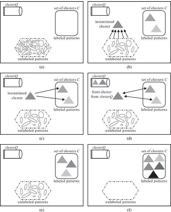
FIGURE 13.2
Illustration of the steps performed in Algorithm 13.1. (a) Initial stage, where the set of clusters C is empty. (b) Step 2, where a cluster is instantiated by using the pattern with longest life span as the generator. The new cluster computes associations with the unlabeled patterns in step 3a of PGA. (c) Step 3b, where the new cluster computes associations with labeled patterns. (d) Step 5, where re-organization of patterns for the clusters that have been put in the clusterQ takes place. (e)ClusterQ is empty at the end of the re-organization step. This state leads to step 6 followed by step 4 and step 2. Further instantiation of new clusters and reorganization takes place till no more unlabeled patterns are left. (f) Termination stage.

Images

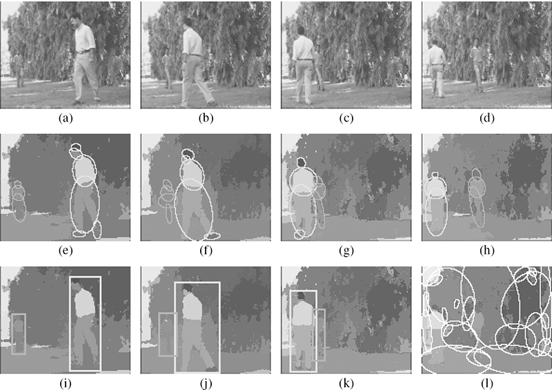
FIGURE 13.3
PGA performance demonstration: (a,e,i) frame 4, (b,f,j) frame 25, (c,g,k) frame 50, and (d,h,l) frame 83. (a–d) Some original frames from a sequence in which two persons are walking in the background of trees. The total length of the sequence is 356 frames. (e–h) Color segmented (clustered) frames produced by the DSCT algorithm. (i–k) The PGA groups foreground clusters, which are marked using rectangles of distinct colors. Blobs that constitute a foreground cluster are highlighted in (e–h) with the same color as that of the bounding rectangle. (l) All other blobs in the scene get grouped into the background cluster. Total number of blob tracks processed is 32 of which 11 were grouped as foreground clusters. Grouping of the background cluster took four iterations of step 5 of PGA, while the two foreground clusters took two iterations each.

13.5 Evaluation of Cluster Identification Using Perceptual Grouping

The output of the perceptual grouping algorithm (PGA) is verified manually and is considered to be correct if the output clusters correspond to meaningful foreground subjects, and no actual foreground region is incorrectly merged with the background or any other foreground cluster. PGA groups the background as a single perceptual cluster; meaningful components in the background are not searched here. Figure 13.3 shows a sequence in which the background has dynamic textures (trees). The color clustering step in the decoupled semantics clustering tree algorithm smooths out the textured background and models all homogeneous color regions as space-time blob tracks. The blobs belonging to the background are more or less static, while those that are part of the two foreground subjects show distinct motion. The PGA identifies three clusters, two foreground clusters and one background cluster, which comprises all the remaining blobs. The decoupled semantics clustering tree algorithm can handle dynamic textures without the need of explicit modeling in contrast to Reference [29].

Images

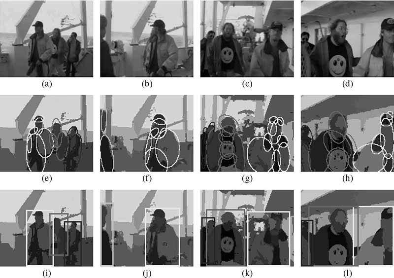
FIGURE 13.4 (See color insert.)
PGA performance demonstration on a sequence from Titanic movie: (a,e,i) frame 77, (b,f,j) frame 103, (c,g,k) frame 142, and (d,h,l) frame 175. (a–d) Original frames, (e–h) PGA-identified foreground blobs on the DSCT color-clustered frame, and (i–l) perceptual clusters marked with the same color as the blobs belonging to the distinct foreground clusters. Note that the person wearing the red jacket, initially seen on the right of the person wearing the yellow jacket, comes to the left starting from frame 110.

Figure 13.4 shows a sequence in which people walk along a passage in a ship. The camera is not static and there are some frames for which the distinct subjects get adjacent to each other and they even change their orientation with respect to each other. As can be seen, the PGA identifies the foreground subjects correctly. Some more representative results of PGA are shown in Figure 13.5. The detailed results and explanations can be found in Reference [1].

Overall, it can be said that the PGA successfully identifies foreground subjects for the class of scenes where the subjects show distinct characteristics compared to the background. The use of node E plays a crucial role in the grouping process when associations like motion similarity and adjacency do not exhibit strongly enough. The output of the PGA crucially depends on what qualifies to be a valid grouping. The factors governing a valid grouping are the observed Gestalt associations, the evidences formulated corresponding to the associations, and the Bayesian network parameters. The PGA reasonably outputs the chunk of pixels that belong to the foreground subjects even in the presence of some inconsistencies in the blob tracks.

Images

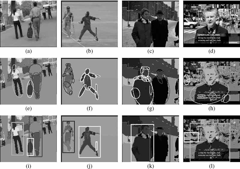
FIGURE 13.5 (See color insert.)
PGA performance demonstration on various scenes: (a–d) original frames in four different scenes, (e–h) identified foreground blobs, and (i–l) perceptual clusters.

Having identified the meaningful objects in the scene foreground, the next problem toward the task of video understanding is to interpret the scene. An interpretation establishes the context in which humans perceive the information about the scene content. The context, among other things, depends significantly on the prominent components in the scene. These ideas and a computational model for perceptual prominence are discussed below.

13.6 Perceptual Prominence

The following describes the proposed principle of perceptual prominence for the subjects in the scene. Prominence refers to cognitive interest in the subjects. The semantics of the scene is closely associated with the prominent subjects, that is, the subjects that deserve attention. Perceptual prominence is different from visual saliency [15], which refers to the identification of salient locations in the scene by the psychophysical sensory mechanisms before any cognitive interpretation is carried out.

Context plays an important role in influencing the prominence measure for scene components (the perceptual clusters). Though a perceptual cluster may be prominent as a stand-alone cluster, the presence of other clusters may establish a context in which it may not be prominent. Hence, it may happen that within a context and an interpretation, one, few, or none of the clusters come out as prominent. The proposed approach to modeling the context is to use perceptual attributes that characterize the context. A contextual attribute captures the distinguishing properties of a cluster with respect to the surrounding background blobs or other foreground clusters present in the scene.

Images

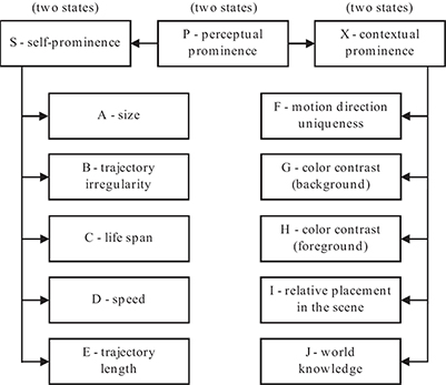
FIGURE 13.6
Belief network [1] for computing the prominence measure for a perceptual cluster c_i.

Prominence can arise in several ways. In many scenes, a subject occupying a position that is in imbalance with the arrangement of the scene components turns out to be prominent. A marked contrast in the appearance of a subject relative to the background or other foreground subjects also directs visual attention, making the subject perceptually prominent. Different interpretations of prominence can be encoded into different prominence models. A specific prominence model denotes a set of perceptual attributes and the way the computed values for the attributes influence the prominence measure for a subject. The choice of a prominence model depends on the type and interpretation of the scene. For example, in a subject-oriented scene, the leading subject generally lasts for a long duration in the shot period and hence is prominent. In surveillance scenes, the subjects appearing for a short span of time or subjects moving in a direction different from other subjects are considered as prominent (deserving attention). Thus, it is possible to formulate one prominence model that identifies subjects showing zigzag motion as prominent, and another model that identifies large-sized subjects with a long life span as prominent, and so on.

The proposed methodology for computing the prominence measure makes use of a belief network, shown in Figure 13.6, which models the prominence of a cluster as a propositional node P. The prominence measure is formulated as the probability computed for the proposition that the cluster is prominent. Each of the nodes P, S, and X takes on two discrete states {isProminent, isNotProminent} for the cluster. The evidences are computed based on a characterization of the perceptual attributes over the entire life span of the subject. All the attributes do not need to be contextual. If none of the perceptual attributes take the context into account, the prominence measure thus computed from the non-contextual (that is, subject specific) attributes is called as the self-prominence measure. In the belief network there are separate nodes for computing measures (that is, probabilities) for self-prominence and contextual prominence. The virtual evidence nodes A through J in the belief network characterize the observation of the perceptual attributes over the entire life span of the subject, and hence are termed as the observation nodes. Instantiation of evidence nodes leads to belief propagation [30] in the Bayesian network and each node updates the posterior probability for its states. The marginalized probability for the positive state of node P is taken as the prominence value. The proposed framework for computing the prominence can be used to model different interpretations of prominence by using an appropriate subset of relevant observation nodes. The computed attribute value is mapped to its contribution toward the prominence by using an evidence function.

13.6.1 Evaluation of Perceptual Prominence

For the sequence shown in Figure 13.7, the proposed grouping algorithm groups the moving subjects (since they have relative motion with respect to the background, they can be grouped without any world knowledge) and the subjects who are stationary (sitting) by making use of the face detector and a skin detector (with vertical oval-shaped blobs signifying a face) and grouping the face regions with the body region below it. Table 13.1 lists the normalized perceptual attributes for four subjects (who are eventually prominent in the scene), along with the computed probability of prominence. A subject with a frontal face gets a higher contribution (at node E) toward its prominence (because a frontal face is generally in focus), compared to non-frontal view faces. The prominence computed for subjects sp1 and sp2 (see Figure 13.7) is high, primarily because of their large life span and size. The motion of the moving subjects, and their higher color contrast compared to the other subjects give them a higher prominence.

A scene can be interpreted in terms of the behavioral analysis of prominent subjects and the mise-en-scène concepts. Cognitive analysis forms the link between the extracted meaningful components and the perceived interpretation of the content. The next section describes the proposed scene interpretation framework.

13.6.2 Scene Categorization Using Perceptual Prominence

Perceptual prominence helps in identifying the meaningful subjects which influence many of the cognitive abstractions from the scene. A scene is characterized here using two broad categories:

Frame-centric scene – A cognitive understanding of a frame-centric scene requires shifting the focus of attention to different spots on the entire frame. A frame-centric scene generally comprises multiple prominent subjects that may be engaged in a group-specific activity or independent activities.
Subject-centric scene – In a subject-centric scene the focus of attention is mainly on the activity of one or two subjects. A subject-centric scene comprises fewer prominent subjects that normally exist for most of the duration of the shot.

Images

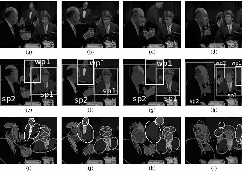
FIGURE 13.7
Perceptual prominence computation for a sequence in which two persons are sitting in a restaurant: (a,e,i) frame 25, (b,f,j) frame 37, (c,g,k) frame 61, and (d,h,l) frame 231. Note other persons sitting in the background and sporadically moving persons, such as the waiter. The foreground subjects are named as sp1 and sp2, for the persons sitting on the right and the left side, respectively; and wp1 and wp2 for the waiter wearing a red uniform and the moving person wearing a dark green coat, respectively.

TABLE 13.1
Perceptual attributes, as depicted in Figure 13.6, computed (and normalized) for four foreground subjects in the sequence shown in Figure 13.7. The normalized perceptual attributes are shown only for prominent subjects (with prominence measure> 0.5). The probabilities computed for self-prominence (S), contextual prominence (X), and the overall prominence (P) are also shown. The prominence computed for subjects sp1 and sp2 is high because of their longer life span and a larger size. The subject sp1 has a frontal face that contributes a higher prominence compared to sp2, which has a side-view face. The prominence for the moving subjects wp1 and wp2 is mainly contributed by their motion and higher color contrast. ©2007 IEEE.

Images

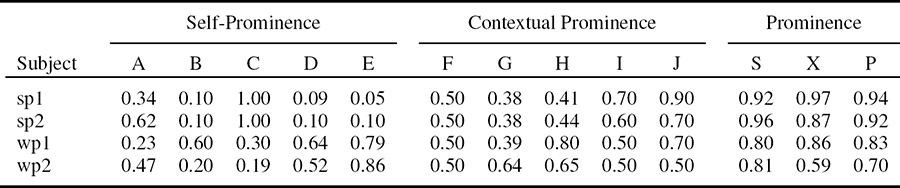
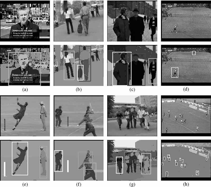
FIGURE 13.8 (See color insert.)
Scene categorization: (a–d) subject-centric scenes, as they all have one or two prominent subjects, which exist throughout the duration of the shot, and (e–h) frame-centric scenes because the subjects in these scenes last only for a small duration in the shot. Prominence values for the subjects taken from left to right: (a) {0.96,0.1}, (b) {0.3, 0.8, 0.95}, (c) {0.8, 0.8, 0.18}, (d) {0.61, 0.66}, and (e–h) values smaller than 0.5 according to the proposed prominence model which includes life span as an attribute.

Examples of subject-centric and frame-centric scenes are given in Figure 13.8. Each of the subject-centric and frame-centric scene category is divided into three subcategories based on the kind of activity exhibited by the subjects:

Independent activity scenes, where a subject follows an independent movement pattern without any influence from the other subjects. The subjects are likely to move in a uniform direction.
Involved activity scenes, where a subject normally moves in response to the movement of the other subjects and are more likely to exhibit an irregular motion compared to those in an independent activity scene. Moreover, the subjects may move in different directions.
No-activity scenes, where the subjects do not show any significant activity. There is little or no motion.

A Bayesian network is a convenient way to model the uncertain relationships between observations and concepts. In the proposed belief network (Figure 13.9) for characterizing the scenes, the nodes G, S, F, V_s, D_s, O_s, V_φ, D_φ, and O_φ are the scene type nodes, and each has two discrete states that correspond to the positive and negative propositions of whether a given scene belongs to the specified type. The nodes shown in dotted rectangles are observation nodes, each contributes to the belief of the scene type node to which it is connected. The node Nsubjects corresponds to the total number of subjects identified in the scene. Three types of prominence models are used, which could identify subjects showing a prominent zigzag motion (subscript zz), or a prominent uniform motion (subscript u) or a prominent no motion (subscript nm). Observations related to these prominent subjects are used in virtual evidence nodes $P_{zz}^{1}, P_{u}^{1}, P_{nm}^{1}, P_{zz}^{2}, P_{u}^{2}, {or P}_{nm}^{2}$ to provide evidences for the relevant scene types.

13.6.3 Evaluation of Scene Categorization

Different scenes are characterized by making use of key mise-en-scène aspects and subject behaviors specific to the scene types. For illustration, the subject behavior observations and scene categorization results are discussed below for a few example scenes:

Cricket: A cricket scene is frame centric, with the subjects generally showing an independent or an involved activity. For a typical scene in which a batsman plays a ball, the camera is moved fast to follow the ball, and hence the subjects exhibit an apparent fast motion in a uniform direction. The subjects show adherence to a prominence model highlighting high-speed motion in a uniform direction.
Tennis: A tennis scene is subject-centric and exhibits an involved activity of the subjects. The subjects show adherence to a prominence model highlighting zigzag motion behavior.

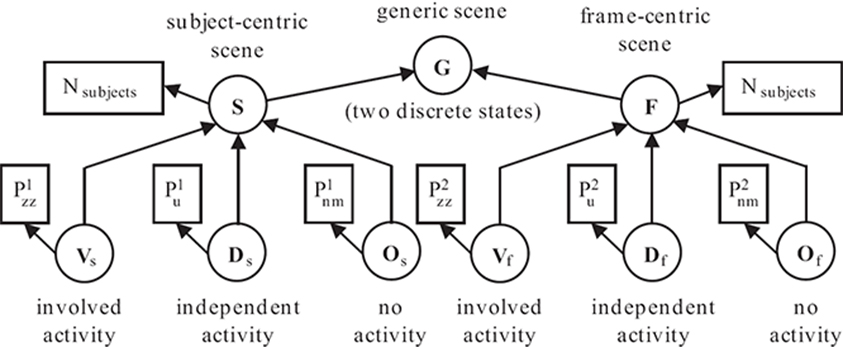
FIGURE 13.9
The belief network for the proposed scene model [1]. ©2007 IEEE.

TABLE 13.2
Scene interpretation on various test videos. Scene 1 evaluated a higher probability for frame centric (0.911) compared to subject centric (0.161). Within frame centric, the subcategory that got the highest probability is involved activity. Hence, this scene is categorized as frame centric with involved activity. Likewise the final categorization of other examples is listed in the table. ©2007 IEEE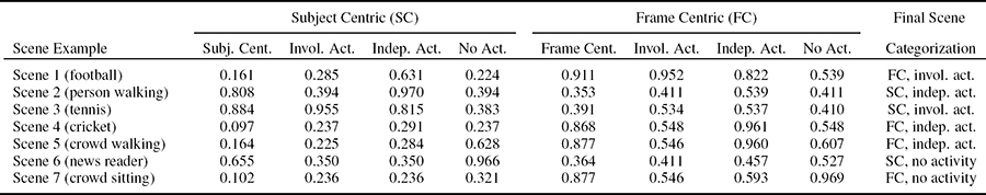

TABLE 13.3
Evaluation of subject- and frame-centric scene categorization on a test set of 215 video shots.

Subject Centric

Frame Centric

Subject Centric

100%

0%

Frame Centric

21%

79%

TABLE 13.4
Evaluation of activity-based scene categorization on a test set of 215 video shots.

Independent Activity

Involved Activity

No Activity

Independent Activity

92%

8%

0%

Involved Activity

19%

77%

4%

No Activity

0%

0%

100%
Football: A football scene is frame centric with involved or independent activity of the subjects. The subjects show adherence to a prominence model highlighting zigzag motion or a uniform direction motion.
News report: A news report has many subject-centric scenes, for example, the scenes where a reporter (a prominent subject) may stand in front of a still background or one having moving objects such as traffic. The foreground subject adheres to a prominence model highlighting subjects with a longer life span and showing no motion.
Crowd scenes: Crowd scenes are frame centric, and generally exhibit independent activity of the subjects. The subjects may be walking in a uniform direction, or may be just sitting.

	Subject Centric	Frame Centric
Subject Centric	100%	0%
Frame Centric	21%	79%

	Independent Activity	Involved Activity	No Activity
Independent Activity	92%	8%	0%
Involved Activity	19%	77%	4%
No Activity	0%	0%	100%

A scene is classified as subject centric or frame centric depending on which of the nodes (S or F) computes a higher belief. A subject-centric scene is further classified as belonging to any of the subcategories that (propositional node) compute the highest belief (among V_s, D_s, and O_s); and likewise for a frame-centric scene. The classification accuracy for a given scene category is computed as the ratio of the number of shots that were correctly classified as belonging to that category to the number of shots that actually belonged to that category. Table 13.2 lists the results of scene interpretation on various example videos. The classification performance is summarized in Tables 13.3 and 13.4. The performance figure is lower for frame-centric scenes; that was mainly because of missed subject detection by the PGA, since generally, such scenes have subjects of small sizes. Further, the involved activity scenes also have a lower classification accuracy and are more likely to get misclassified as independent activity scenes. This happens mostly when the subject life span is small or the shot duration is small, so that the subject motion appears more or less uniform and in similar directions. As it can be seen, the various scene examples have been correctly interpreted into the scene hierarchy. Extensibility of the proposed interpretation framework to incorporate other classes of scenes requires formulating appropriate observations (evidences) for characterizing the scenes.

13.7 Perceptual Grouping with Learned Object Models

This section explores the use of learned object-model knowledge with the perceptual organization process. A framework, which not only performs detection of foreground objects but also recognizes the object category, is proposed. The advantages of the add-on grouping evidences, as contributed by the object models for a more robust perceptual organization in the spatiotemporal domain, are demonstrated. The object is modeled as a pictorial structure [31], [32] since this kind of representation involves modeling an object as a composition of parts. It offers a probabilistic model, which allows computing the likelihood of the part or the object as a whole in the process of grouping. This in turn provides a scheme for object recognition through a grouping process in a video sequence. Using perceptual grouping in spatiotemporal domain avoids the need of bootstrapping, that is, having a correct recognition of the object in the first frame. Further, it gathers grouping evidences from all the frames of a video, and is thus more reliable in detecting specific (with known models) objects as well as general objects.

Section 13.7.1 describes the proposed object model formulated as pictorial structures. The perceptual grouping algorithm that uses the domain knowledge is discussed in Section 13.7.4. The experimental results are reported in Section 13.7.5.

13.7.1 Object Model as a Pictorial Structure

Consider an object with parts v₁, v₂,..., v_n, where each part v_i has a configuration-label specified as l_i on a common coordinate frame. This label is formulated as l_i = (x_i, y_i, θ_i, σ_i), where (x_i, y_i) denotes the location, θ_i is the orientation, and σ_i is the scale at which the object part occurs in the image plane. An instance of the pictorial structure model for an object can be defined using its part-configuration parameters λ = {l₁,l₂,..., l_n} and the part-appearance parameters a = {a₁,a₂,.., a_n}, where the subscript indicates the part index. The Bayesian formulation is adopted for pictorial structures as given in Reference [32]. Let n_P be the set of parts that together comprise the object model. Let D_i denote the image region of the ith part. The posterior distribution from the model parameters can be defined as follows:

$P (a, l | D) \propto \prod_{i = 1}^{i = n_{p}} \frac{P (D_{i} | a_{i})}{P (D_{i} | a_{b g})} \exp (- \sum_{j \neq i} Ψ (l_{i}, l_{j})) (13.4)$

where Ψ(l_i, l_j) is the potential between parts v_i and v_j, and a_i and a_bg are appearance parameters for part v_i and background, respectively. The part labels which maximize the posterior probability are taken as the best fit for the pictorial structure model.

13.7.2 Learning the Object Model

An object model is learned in terms of the configuration of the body parts and the appearance of each of the body parts. Considering analogy with a Markov random field model, each object part is considered to be a site. Configuration compatibility of the two parts is formulated as the potential between them. To compute a continuous measure of conformance of an observed configuration with the expected (true) configuration, the relative configuration of the two parts is modeled using parameters h_{i j} = {length,orientation} of a hypothetical line joining the centroid of the parts v_i and v_j. Then, the distribution of the two parameters is modeled as a mixture of Gaussians.

The potential Ψ(l_i, l_j) between two parts is defined as

$Ψ (l_{i}, l_{j}) = \sum_{x = 0}^{C} w_{x} \frac{{| \sum_{x_{i j}}^{- 1} |}^{1 / 2}}{2 π} \exp (- \frac{1}{2} {(h_{i j} - μ_{x_{i j}})}^{t} \sum_{x_{i j}}^{- 1} (h_{i j} - μ_{x_{i j}})) (13.5)$

where C is the number of Gaussians, w_x is the weight given to the xth Gaussian modeled with covariance matrix ∑_{x_ij} and mean μ_{x_ij}. While learning the potential, it was found that the Gaussian mixture model learning algorithm gives the maximum log-likelihood score (sum of log-likelihoods over all the training samples) for a mixture of two Gaussians.

13.7.3 Formulation of Appearance Parameters for Object Parts

An object part may have fine distinguishing image features and may also contain important information in lower frequencies. It is desirable that the visual attributes provide a representation of the appearance that is jointly localized in space, frequency, and orientation. For this purpose, a wavelet transform is used to decompose the image into various subbands localized in orientation and frequency. The subbands represent different frequencies in horizontal, vertical, and diagonal orientations, and in multiple resolutions. The coefficients within a subband are spatially localized as well. Here, a three-level wavelet decomposition using Haar filter is performed. Level 1 describes the lowest octave of frequency, whereas each subsequent level represents the next higher octave of frequencies.

Algorithm 13.3 summarizes the steps in learning the object-part detector using the appearance attributes formulated on wavelet coefficients. Note that the attribute histograms need to be learned on a fairly large labeled dataset in order to be representative of the object and non-object categories.

ALGORITHM 13.3 Learning of the object-part detector using the appearance attributes formulated on wavelet coefficients.

Decompose the known object region (rectangular) into subwindows.
Within each subwindow (w_x, w_y), model the joint statistics of a set of quantized wavelet coefficients using a histogram. Several such histograms are computed, each capturing the joint distribution of a different set of quantized wavelet coefficients. Here, 17 such histograms are obtained. The coefficient sets are formulated as given in Reference [33].
A histogram is a nonparametric statistical model for the wavelet coefficients evaluated on the subwindow. Hence, it can be used to compute the likelihood for an object being present or not being present. The detector makes its decision using the likelihood ratio test:

$\frac{\prod_{w_{x}, w_{y}} \prod_{k = 1}^{17} P_{k} ({histogram}_{k} (w_{k}, w_{y}), w_{x}, w_{y}) | object)}{\prod_{w_{x}, w_{y}} \prod_{k = 1}^{17} P_{k} ({histogram}_{k} (w_{k}, w_{y}), w_{x}, w_{y}) | non-object)} > λ$

where the outer product is taken over all the subwindows (w_x, w_y) in the image region of the object. The threshold λ is taken as P(non–object)/P(object), as proposed in Reference [33].

13.7.4 Spatiotemporal Grouping Model with Object Model Knowledge

The spatiotemporal grouping framework relies on making use of evidences formulated on the observed associations amongst the patterns. In Figure 13.1, the evidence contributed by a pattern signifies its association strength with the rest of the grouping. The virtual evidence nodes v_e1, v_e2,..., v_en contribute evidences corresponding to the conformance of a putative grouping of blob patterns to a known object model. A virtual evidence v_ei computes the grouping probability of a pattern p_i with the rest of the patterns in the grouping, given the knowledge of the object model. A pattern p_i may exhibit only a partial overlap with an object. Assuming an object O_m comprising of $v_{1}^{m}, v_{2}^{m}, \dots, v_{n}^{m}$ parts, it is necessary to find whether p_i overlaps with any of the object parts. Algorithm 13.4 summarizes the steps of this procedure.

ALGORITHM 13.4 Searching for overlaps between pattern p_i and object parts.

Define a search window (around the pattern) that is larger than the size of the pattern.
At all locations (w_x, w_y) within that window do a search for each as yet undetected object part at three different scales. An object part is taken to be detected correctly if its posterior (Equation 13.4) is above a threshold. Note that when using Equation 13.4, the product index i is taken over the n_D parts that have been already detected up to this step.
The overlap of p_i with object part(s) provides a measure of the degree to which the pattern belongs to the object. If the fractional overlap (in number of pixels) of p_i with the object is found to be more than 30% of the area of p_i, the pattern is said to have a qualified overlap with the object O_m.
Step 3 is repeated for all the frames F_pi for which the pattern (blob track) p_i exists. The association strength of the pattern p_i with the object O_m is formulated as $(Σ_{\forall f \in F_{p_{i}}} α_{p_{i}}^{f}) / F_{p_{i}}$ , where $α_{p_{i}}^{f} = 1$ if p_i has a qualified part match in the frame f, and $α_{p_{i}}^{f} = 0$ otherwise. This association measure gets computed in the range [0,1] and is taken as the probabilistic evidence contributed at nodes v_e1, v_e2,..., v_en, in favor of the putative cluster.

13.7.4.1 Grouping-Cum Recognition

Having formulated the grouping evidence for a pattern using the object-model knowledge, the following lists the steps of the grouping-cum recognition algorithm. Using object model knowledge requires an extra procedure (step 3 in Algorithm 13.5) to be added to the grouping algorithm discussed in Section 13.4.1. The node E is used to provide the object model-based grouping evidences when the cluster c_j has been associated with a hypothesized object-class label. The object class label is chosen depending on the object part to which the generator pattern matches. If the generator pattern does not match with any object part, then it would initiate a general grouping without any object class label. Given a set of object models $O = {O_{1}, O_{2}, \dots, O_{s}}$ and a set of patterns P ={p₁, p₂,..., p_n}, the proposed algorithm outputs the set of perceptual clusters C ={c₁,c₂,..., c_r}.

ALGORITHM 13.5 Perceptual grouping-cum recognition.

Input: Set of object models $O = {O_{1}, O_{2}, \dots, O_{s}}$ and a set of patterns P = {p₁, p₂,..., p_n}.

Output: Perceptual clusters with a labeled object class (if any).

Initialize the set of clusters C ={}. Hence, $J_{s c e n e} = 0$ . Instantiate a queue, clusterQ, to be used for storing the clusters. Initially none of the patterns have any cluster label.
If all the patterns have cluster labels and the clusterQ is empty, then exit. Otherwise, instantiate a new cluster if there are patterns in set C that do not have any cluster label. From among the unlabeled patterns, pick up the one that has the maximum life span. This pattern is taken as the generator pattern for the new cluster c_new.
The generator may or may not be a part of any of the objects in set $O$ . Define a search region around the generator and look for possible parts of any of the objects, as depicted in Figure 13.10. The object part(s) which compute (by virtue of their appearance) the a posteriori probability in Equation 13.4 to be greater than a threshold are considered as present in the search region. The generator pattern is labeled as belonging to the object with which it shares the maximum overlap (in terms of number of pixels). The correctness of the object label is further verified by checking its consistency in five other frames in which the generator blob exists. Once an object label (say, O_m) has been associated with the generator, the node E is used to provide a probability of a pattern being a part of the object O_m. If the generator pattern cannot be associated with any object label from set $O$ , the node E is not used in the grouping model. The cluster formed by such a generator corresponds to a general grouping without any specific object tag. Moreover, such a grouping would use only the general associations for grouping.
(a) Compute associations of the generator pattern of c_new with the unlabeled patterns. An unlabeled pattern p_i is added to the cluster c_new if P(p_i ∪ c_new)> 0.5. Repeat this step till no more unlabeled patterns get added to c_new. Any unlabeled patterns that exist now are the ones that do not form a valid grouping with any of the existing clusters.

(b) Compute associations of the generator pattern of c_new with the labeled patterns of other clusters. If there are patterns, say, p_k (of another cluster, say, c_j) that form a valid grouping with c_new, that is, P(p_k ∪ c_new)> 0.5, then put c_new and c_j into the clusterQ if they are not already there inside it.
If the clusterQ is empty, go to step 2. Otherwise, take the cluster at the front of the clusterQ. Let this cluster be cf.
Pick a pattern, say, p_i, of the cluster c_f. The pattern p_i is considered to be a part of, one by one, every cluster in the set C. The association measures between p_i and a cluster c_j need to be recomputed if c_j has been updated. For each cluster c_j in C, compute the grouping probability for the putative grouping {p_i ∪ c_j}. If the grouping {p_i ∪ c_j} is valid (that is, P(p_i ∪ c_j)> 0.5), the change in the scene grouping saliency is noted as δ_S = P(p_i ∪ c_j) − P(c_j). The pattern p_i is labeled with the cluster (say, c_m) for which δ_S computes to the highest value. If c_m is not c_f, then put c_m into the clusterQ, if it is not already inside it. Repeat step 4 for all the patterns in c_f.
If any pattern in c_f changes its label as a result of step 5, then go to step 4. If none of the patterns changes its label, remove the front element of the clusterQ and go to step 4.

Apart from step 3 (which gives an object label to the generator), the algorithm follows the steps in the original PGA. The iterative process terminates when the pattern labels have stabilized. Each cluster has a label of the object class to which it belongs.

Images

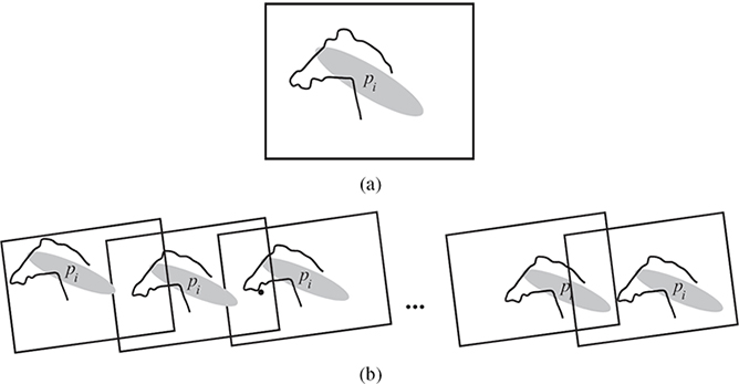
FIGURE 13.10
Illustration of the steps performed in Algorithm 13.2: (a) a bounding box defined around a pattern p_i, (b) the consistency of the overlap of the object part with the pattern p_i is established for a sequence of frames.

13.7.5 Evaluation of Perceptual Grouping with Object Models

The models were trained for two object categories: cows and horses. For the purpose of learning the appearance attribute histograms for the object parts and the non-object regions, the appearance features were computed for each object part for about 650 images, sampled from cow/horse videos. A large training set is needed since the skin texture/color has substantial variations within certain animal categories. The features were also learned for the mirror images of the object regions. To minimize the classification error, different weights were used for the different attributes [33]. The Gaussian mixture model distribution of configuration for each pair of object parts was also learned. The appearance attribute histograms for non-object regions were learned from about 1200 random images that did not have the object.

The experiment has helped to establish two advantages offered by the perceptual grouping process through an effective use of object model knowledge. First, once an object part has been reliably detected (with high probability), other (computationally costly) evidences, such as adjacency and cluster-bias, do not need to be gathered for all the frames since an object model is a very strong grouping evidence that would allow grouping of only the blobs that overlap with some part of the same object. Second, there are scenes in which the foreground subjects do not show a distinct motion with respect to the background. For such a case, the general grouping criteria would group all the blobs in the scene to output a single cluster having both the background and the foreground. Such failure cases are shown to be successfully handled by the use of object models that provide a stronger grouping evidence to compensate for the (non-exhibited) general grouping evidences. Searching an object part around a blob pattern is a costly operation; however, it needs to be done only once, and not in every iteration of the grouping algorithm. Moreover, it can be computed on a few frames (around five) and not on all the frames of the blob track, since a consistent overlap of the blob with an object part on a few frames can be taken as an indicator that the blob belongs to the object region. It was observed that certain object parts get missed by the detectors when a large object motion causes blur in the object appearance, since the appearance gets confused with the background. For such cases, the generic grouping evidences play the major role in the grouping process.

Images

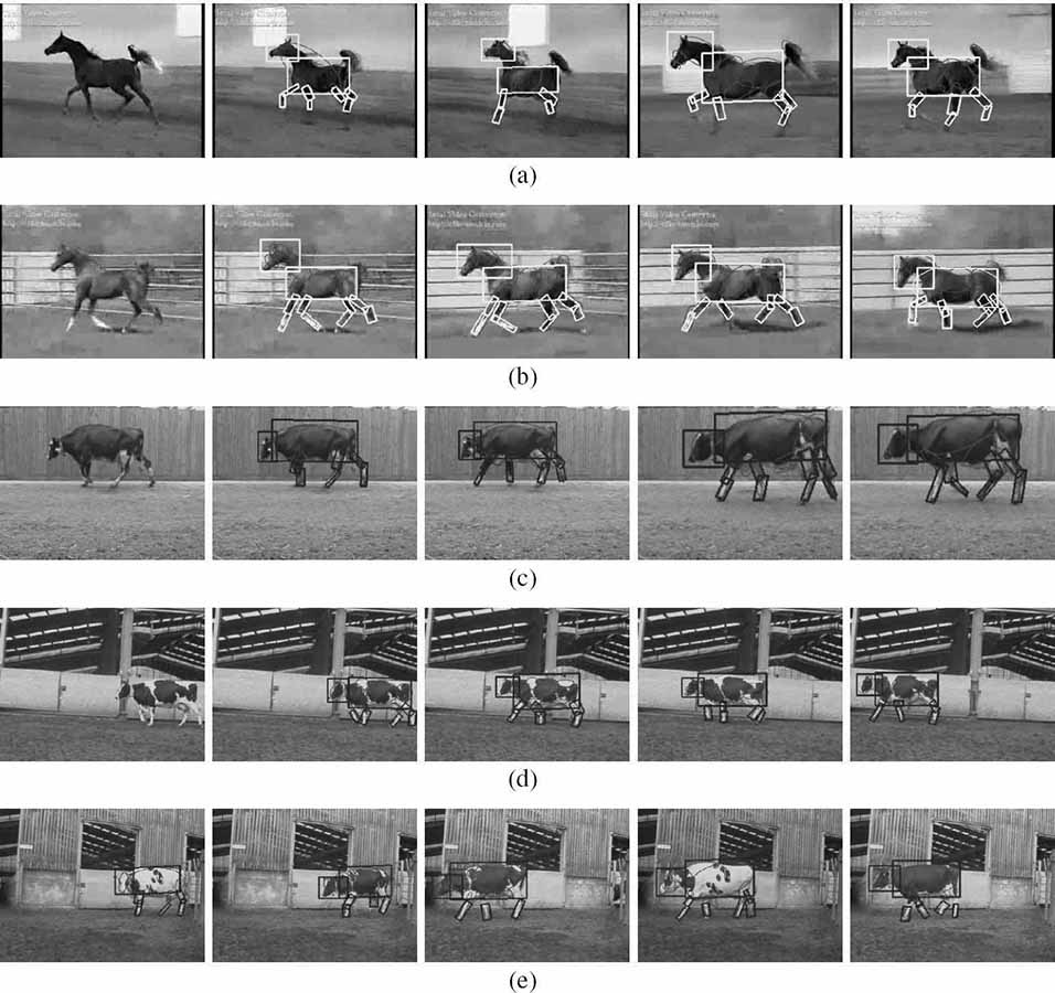
FIGURE 13.11 (See color insert.)
Results obtained for various horse and cow videos. Probability at node E: (a) 0.814, (b) 0.795, (c) 0.910, (d) 0.935, and (e) 0.771, 0.876, 0.876, 0.800, and 0.911 for different videos with the object model cow.

Figure 13.11 presents the results of grouping with learned object models. Namely, Figures 13.11a and 13.11b show the result of applying the grouping algorithm to test videos of a horse galloping in a barn. The camera is panning and the background remains almost constant. Thus, blob patterns belonging to both the object and the background have almost no motion. Hence, simple generic grouping (using motion similarity, adjacency, and so on), when applied to such a video, fails to successfully cluster the patterns into meaningful organizations and clusters all patterns into one large cluster. This situation is resolved in the proposed model-guided perceptual grouping scheme, where the evidence from the object model knowledge is used to correctly groups the object region blobs into a separate cluster. In the presented figures, the recognized object parts are shown as rectangles overlaying the blobs belonging to the horse region.

Figures 13.11c to 13.11e show results on various test videos with cows of very different textures and appearances. The algorithm is successfully able to cluster all the blob patterns belonging to the cows and detect and recognize parts around the patterns (shown as rectangles).

The proposed algorithm has demonstrated the benefits of using object models as domain knowledge to assist, in both computational speed-up and detection accuracy, in the perceptual organization process applied to videos. The results have been presented on two object classes; and as future work, the goal will be to demonstrate use of object models for correctly grouping multiple foreground-objects, which could be sharing similar motion and adjacency in the video frames.

13.8 Conclusion

This chapter presented unsupervised techniques to identify objects that show distinct perceptual characteristics with respect to the background. The decoupled semantics clustering tree methodology is an unsupervised clustering tool for analyzing video data. It employs a decoupled clustering scheme applied to feature subspaces with different semantics for the six-dimensional heterogeneous feature space of video to model the homogeneous color regions in a video scene as temporal tracks of two-dimensional blobs.

The space-time blob tracks (simpler primitives or visual patterns) obtained by the decoupled semantics clustering tree methodology are subsequently grouped together to compose the meaningful objects. A perceptual grouping scheme for the spatiotemporal domain of video was proposed to complete this task. The grouping scheme relies on a specified grouping model. This model makes use of inter-pattern association measures motivated from the Gestalt law of common fate, which states that the entities having a coherent behavior in time are likely to be parts of the same organization. Temporal coherence is established with the premise that time is not an added dimension to the data to be grouped, but it is an added dimension to the grouping such that the grouping should maintain coherence in time. This chapter presented formulations for novel association measures that characterize the temporal coherence between primitives in order to group them into salient spatiotemporal clusters, termed as perceptual clusters. The foreground perceptual clusters correspond to the subjects in the scene. The grouping saliency was defined as a measure of goodness of a grouping, and quantified as a probabilistic measure computed using a Bayesian network model. The perceptual grouping problem was formulated as an optimization problem. The perceptual grouping algorithm (PGA) maximizes the overall scene saliency to a local maximum and obtains a set of perceptual clusters. The PGA successfully identifies foreground subjects for the class of scenes where the subjects show distinct characteristics compared to the background. As part of future work it would be interesting to explore if such grouping models could be learned. This would mean learning the structure of the grouping belief network, the optimal set of association attributes to be used, and their relative influence in the computation of grouping saliency. This chapter also demonstrated the use of learned object models as domain knowledge to assist in grouping as well as recognition of the object class instances in a video shot. Use of object models was also shown to assist in computational speed-up and improved detection accuracy in the perceptual organization process.

The problem of general scene characterization was explored by making use of different interpretation models to detect and analyze the meaningful components in the scene. A computable model for characterizing a video scene into two broad categories was designed. The two categories are subject-centric scenes, which have one or few prominent subjects, and frame-centric scenes, in which none of the objects can be attributed a high prominence and hence the overall activity depicted in a sequence of frames is the subject of interest. In addition, a novel concept of perceptual prominence for the identified subjects was proposed. Perceptual prominence has been motivated from film grammar that states that human understanding of the scene depends on the characteristics of scene components focused on. It is an extension of the concept of saliency to the cognitive level. Further, it depends on chosen interpretation of prominence, as different subjects may turn out to be prominent when using different interpretations of prominence. Prominence is interpreted by formulating an appropriate model based on attributes that commonly influence human judgment about meaningful subjects. Here, empirical prominence models for formulating perceptual evidences for various types of scenes were used. The attribute specifications were parametrized into different prominence models that signify different interpretations of prominence. A set of perceptual and contextual attributes that influence the prominence were described and a methodology that uses the perceptual attributes and computes a value signifying the prominence was developed. Moreover, a taxonomy of interpretation of video scenes was generated; each of the subject-centric and frame-centric scene classes was divided into three subcategories (independent activity scenes, involved activity scenes, and no-activity scenes), based on the kind of activity exhibited by the subjects. Presented experimental results established the effectiveness of the proposed perceptual attribute-based prominence formulation and showed that such attributes indeed have a direct relationship to many of the cognitive abstractions from a video scene. The scene interpretation framework can be extended to incorporate other classes of scenes by formulating appropriate observations (evidences) for the more specific scene classes.

Acknowledgment

Figure 13.9 and Tables 13.1 and 13.2 are reprinted from Reference [1] with the permission of IEEE.

References

[1] G. Harit and S. Chaudhury, “Video shot characterization using principles of perceptual prominence and perceptual grouping in spatio-temporal domain,” IEEE Transactions on Circuits and Systems for Video Technology, vol. 17, no. 12, pp. 1728–1741, December 2007.

[2] D. Bordwell and K. Thompson, FILM ART An Introduction. New York, USA: McGraw-Hill Higher Education, 2001.

[3] D.D. Hoffman and B.E. Flinchbaugh, “The interpretation of biological motion,” Biological Cybernatics, vol. 42, no. 3, pp. 195–204, 1982.

[4] M. Nicolescu and G. Medioni, “Perceptual grouping from motion cues using tensor voting in 4-D,” in Proceedings of the 7th European Conference on Computer Vision, Copenhagen, Denmark, May 2002, vol. 3, pp. 303–308.

[5] A. Verri and T. Poggio, “Against quantitative optic flow,” in Proceedings of the First International Conference on Computer Vision, London, UK, June 1987, pp. 171–180.

[6] R. Nelson and J. Aloimonos, “Towards qualitative vision: Using flow field divergence for obstacle avoidance in visual navigation,” in Proceedings of the Second International Conference on Computer Vision, Tarpon Springs, FL, USA, December 1988, pp. 188–196.

[7] M. Shah, K. Rangarajan, and P.S. Tsai, “Generation and segmentation of motion trajectories,” in Proceedings of 11th International Conference on Pattern Recognition, The Hague, The Netherlands, September 1992, pp. 74–77.

[8] S. Sarkar, “Tracking 2D structures using perceptual organization principles,” in Proceedings of the International Symposium on Computer Vision, Coral Gables, FL, USA, November 1995, pp. 283–288.

[9] S. Sarkar, D. Majchrzak, and K. Korimilli, “Perceptual organization based computational model for robust segmentation of moving objects,” Computer Vision and Image Understanding, vol. 86, no. 3, pp. 141–170, June 2002.

[10] S.E. Palmer, “The psychology of perceptual organization: A transformational approach,” in Human and Machine Vision, J. Beck, B. Hope, and A. Rosenfeld (eds.), New York, USA: Academic Press, 1983, pp. 269–339.

[11] E.L.J. Leeuwenberg, “Quantification of certain visual pattern properties: Salience, transparency, similarity,” in Formal Theories of Visual Perception, E.L.J. Leeuwenberg and J.F.J.M. Buffart (eds.), New York, USA: Wiley, 1978, pp. 277–298.

[12] S. Sarkar and K.L. Boyer, Computing Perceptual Organization in Computer Vision. River Edge, NJ, USA: World Scientific, 1994.

[13] D.G. Lowe, Perceptual Organization and Visual Recognition. Boston, MA, USA: Kluwer Academic Publishers, 1985.

[14] A. Shashua and S. Ullman, “Structural saliency: The detection of globally salient structures using locally connected network,” in Proceedings of the Second International Conference on Computer Vision, Tarpon Springs, FL, USA, December 1988, pp. 321–327.

[15] L. Itti, Models of Bottom-Up and Top-Down Visual Attention. PhD thesis, California Institute of Technology, Pasadena, CA, USA, 2000.

[16] D.T. Lawton and C.C. McConnell, “Perceputal organization using interestingness,” in Proceedings of the Workshop on Spatial Reasoning and Multi-Sensor Fusion, St. Charles, IL, USA, October 1987, pp. 405–419.

[17] M. Wertheimer, “Laws of organization in perceptual forms,” in A Sourcebook of Gestalt Psychology, Harcourt, Brace and World, 1938, pp. 71–88.

[18] K. Koffka, Principles of Gestalt Psychology. New York, USA: Harcourt, 1935.

[19] W. Kohler, Gestalt Psychology. New York, USA: Liveright Publishing Corporation, 1929.

[20] I. Rock and S. Palmer, “The legacy of Gestalt psychology,” Scientific American, vol. 263, no. 6, pp. 84–90, December 1990.

[21] S. Sarkar and K.L. Boyer, “Perceptual organization in computer vision: A review and a proposal for a classificatory structure,” IEEE Transactions on Systems, Man, and Cybernetics, vol. 23, no. 2, pp. 382–399, March 1993.

[22] S.F. Chang, W. Chen, H.J. Meng, H. Sundaram, and D. Zhong, “A fully automated content-based video search engine supporting spatiotemporal queries,” IEEE Transactions on Circuits and Systems for Video Technology, vol. 8, no. 5, pp. 602–615, September 1998.

[23] J. Sivic and A. Zisserman, “Video Google: A text retrieval approach to object matching in videos,” in Proceedings of International Conference on Computer Vision, Nice, France, October 2003, vol. 2, pp. 1470–1477.

[24] N. Vasconcelos and A. Lippman, “Toward semantically meaningful feature spaces for the characterization of video content,” in Proceedings of the IEEE International Conference on Image Processing, Washington, DC, USA, October 1997, vol. 1, pp. 25–29.

[25] B. Adams, C. Dorai, and S. Venkatesh, “Toward automatic extraction of expressive elements from motion pictures: Tempo,” IEEE Transactions on Multimedia, vol. 4, no. 4, pp. 472–481, December 2002.

[26] H. Sundaram and S.F. Chang, “Computable scenes and structures in films,” IEEE Transactions on Multimedia, vol. 4, no. 4, pp. 482–491, December 2002.

[27] G. Harit and S. Chaudhury, “Clustering in video data: Dealing with heterogeneous semantics of features,” Pattern Recognition, vol. 39, pp. 789–811, May 2006.

[28] D. DeMenthon and R. Megret, “Spatio-temporal segmentation of video by hierarchical mean shift analysis,” Technical report, LAMP-TR-090, University of Maryland, College Park, MD USA, July 2002.

[29] Y. Sheikh and M. Shah, “Bayesian modeling of dynamic scenes for object detection,” IEEE Transactions on Pattern Analysis and Machine Intelligence, vol. 27, no. 11, pp. 1778–1792, November 2005.

[30] R.E. Neapolitan, Probabilistic Reasoning in Expert Systems: Theory and Algorithms. New York, USA: John Wiley and Sons, 1990.

[31] P. Felzenszwalb and D. Huttenlocher, “Efficient belief propagation for early vision,” in Proceedings of the IEEE International Conference on Computer Vision and Pattern Recognition, Washington, DC, USA, June 2004, pp. 261–268.

[32] M.P. Kumar, P.H.S. Torr, and A. Zisserman, “Extending pictorial structures for object recognition,” in Proceedings of the British Machine Vision Conference, London, UK, September 2004, vol. 2, pp. 789–798.

[33] H. Schneiderman and T. Kanade, “A statistical method for 3D object detection applied to faces and cars,” in Proceedings of the IEEE International Conference on Computer Vision and Pattern Recognition, Hilton Head, SC, USA, June 2000, vol. 1, pp. 746–751.

..................Content has been hidden....................

You can't read the all page of ebook, please click here login for view all page.

Table of Contents for 13 Perceptually Driven Video Shot Characterization

Create new playlist

Sign In

Sign Up

Table of Contents for
13 Perceptually Driven Video Shot Characterization