11 Perceptual Color Descriptors

Color in general plays a crucial role in today’s world. Color alone can influence the way humans think, act, and even react. It can irritate or soothe eyes, create ill-tempers, or result in loss of appetite. Whenever used in a right form, color can save on energy; otherwise, it can cause detrimental effects. Particularly, the color composition of an image can turn out to be a powerful cue for the purpose of content-based image retrieval (CBIR), if extracted in a perceptually oriented way and kept semantically intact. Furthermore, the color structure in a visual scenery is robust to noise, image degradations, changes in size, resolution, and orientation. Eventually, most of the existing CBIR systems use various color descriptors in order to retrieve relevant images (or visual multimedia material); however, their retrieval performance is usually limited especially on large databases due to lack of discrimination power of such color descriptors. One of the main reasons for this is because most of such systems are designed based on some heuristics or naive rules that are not formed with respect to what humans or more specifically the human visual system (HVS) finds relevant in terms of color similarity. The word relevance is described as “the ability (as of an information retrieval system) to retrieve material that satisfies the needs of the user.” Therefore, it is of decisive importance that human color perception is respected while modeling and describing any color composition of an image. In other words, if and only when a particular color descriptor is designed based entirely on HVS and human color perception rules, further discrimination power and hence certain improvements in the retrieval performance can be achieved.

Accordingly, the study of human color perception and similarity measurement in the color domain become crucial and there is a wealth of research performed in this field. For example, Reference [1] focused on the utilization of color categorization (termed as focal colors) for CBIR purposes and introduced a new color matching method, which takes human cognitive capabilities into account. It has exploited the fact that humans tend to think and perceive colors only in eleven basic categories. Reference [2] performed a series of psychophysical experiments, analyzing how humans perceive and measure similarity in the domain of color patterns. These experiments resulted in five perceptual criteria (so-called basic color vocabulary), which are important for comparing the color patterns, as well as a set of rules (so-called basic color grammar), which are governing the use of these criteria in similarity judgment. One observation worth mentioning here is that the human eye cannot perceive a large number of colors at the same time, nor is it able to distinguish similar colors well. At the coarsest level of judgment, the HVS judges similarity primarily using dominant colors, that is, few prominent colors in the scenery. Henceforth, the two rules are particularly related for modeling the similarity metrics of the human color perception. The first one indicates that the two color patterns that have similar dominant colors (DCs) are perceived as similar. The second rule states that two multicolored patterns are perceived as similar if they possess the same (dominant) color distributions regardless of their content, directionality, placement, or repetitions of a structural element.

It is known that humans focus on a few dominant colors and their spatial distributions while judging the color similarity between images. Humans have the ability to extract such a global color view out of a visual scenery, irrespective of its form, be it a digital image or a natural three-dimensional view. However, accomplishing this is not straightforward while dealing with digital images for CBIR purpose. In a standard 24-bit representation, there is a span of 16 million colors, which can be assigned on thousands of individual pixels. Such a high-resolution representation might be required for current digital image technologies; however, it is not too convenient for the purpose of describing color composition or performing a similarity measurement based on the aforementioned perception rules. Nevertheless, it is obvious that humans can neither see individual pixels, nor perceive even a tiny fracture of such a massive amount of color levels, and thus it is crucial to perform certain steps in order to extract the true perceivable elements (the true DCs and their global distributions). In other words the imperceivable elements, called here as outliers, which do not have significant contribution or weight over the present color structure, in both color and spatial domain, should be suppressed or removed. Recall that according to two color perception rules presented in Reference [3], two images that are perceived as similar in terms of color composition have similar DC properties; however, the color properties of their outliers might be entirely different and hence this can affect (degrade, bias, or shift) any similarity measurement if not handled accordingly. For example, popular perceptual audio coding schemes, such as MP3 and AAC [4], maximize the coding efficiency by removing outlying sound elements, that humans cannot hear, in both time and frequency domains and thus more bits can be spent for the dominant sound elements. In a similar fashion, the outliers both in color and spatial domain should be removed for description efficiency. Henceforth, this chapter mainly focuses on a systematic approach to extract such a perceptual color descriptor and efficient similarity metrics to achieve the highest discrimination power possible for color-based retrieval in general-purpose image databases.

Furthermore, one can also note that human color perception is strongly dependent on the variations in their adjacency, thus the spatial distribution of the prominent colors should also be inspected in a similar manner. The color correlogram [5], [6], is one of the most promising approaches in the current state of art, which is a table where the kth entry for the color histogram bin pair (i, j) specifies the probability of finding a pixel of color bin j at a distance k within a maximum range d from a pixel of color bin i in an image I with dimensions W × H quantized with m colors. Accordingly, Reference [7] conducted a comprehensive performance evaluation among several global/spatial color descriptors for CBIR and reported that the correlogram achieves the best retrieval performance among many others, such as color histograms, color coherence vector (CCV) [8], color moments, and so on. However, it comes along with many infeasibility problems, such as its massive memory requirement and computational complexity. This chapter shall first present a detailed feasibility analysis for the correlogram in the next section. Apart from the aforementioned feasibility problems, using the probability alone makes the descriptor insensitive to the dominance of a color or its area (weight) in the image. This might be a desirable property in finding the similar images, such as images that are simply zoomed [6], and hence the color areas significantly vary while the distance probabilities do not. On the other hand, it also causes severe mismatches especially in large databases, since the probability of the pairwise color distances might be the same or close independent of their area and hence regardless of their dominance (whether they are DCs or outliers). Therefore, in this chapter, stemming from the earlier discussions, a perceptual approach will be presented in order to overcome the shortcomings of the correlogram, namely, its lack of perceptuality and infeasibility. This chapter shall present a color descriptor that utilizes a dynamic color clustering and extracts the DCs present in an image in order to bring in the nonexistent perceptuality to the correlogram. Global color properties are thus obtained from these clusters. Dominant colors are then back-projected onto the image to capture the spatial color distribution via a DC-based correlogram. Finally, a penalty-trio model combines both global properties extracted from the DCs and their spatial similarities obtained through the correlogram, forming a perceptual distance metric.

The perceptual correlogram, although an efficient solution for the lack of color perceptual model and computational infeasibility, cannot yet properly address the outlier problem. In order to remove the spatial outliers and to secure the global (perceptual) color properties, one alternative is to apply nonlinear filters (for example, median or bilateral [9]). However, there would be no guaranty that such a filter will remove all or the majority of the outliers and yet several filter parameters are needed to be set appropriately for an acceptable performance, which is not straightforward to do so, especially for large databases. Instead, a top-down approach is adopted both in extracting DCs and modeling their global spatial distribution. This approach is in fact phased from the well-known Gestalt rule of perception [10] formulated as “humans see the whole before its parts.” Therefore, the method strives to extract what is the next global element both in color and spatial domain, which are nothing but the DCs and their spatial distribution within the image. In order to achieve such a global spatial representation within an image, starting from the entire image, quad-tree decomposition is applied to the current (parent) block only if it cannot host the majority of a particular DC; otherwise, it is kept intact (non-decomposed) representing a single, homogeneous DC presence in it. So, this approach tries to capture the whole before going through its parts, and whenever the whole body can be perceived with a single DC, it is kept as is. Hence outliers can be suppressed from the spatial distribution and furthermore, the resultant (blockwise) partitioned scheme can be efficiently used for a global modeling and due description of the spatial distribution. Finally, a penalty-trio model uses both global and spatial color properties, and performs an efficient similarity metric. After the image is (quad-tree) decomposed, this global spatial distribution is then represented via inter-proximity statistics of the DCs, both in scalar and directional modes. These modes of spatial color distribution (SCD) can both describe the distribution of a particular DC with itself (auto-SCD) and with other DCs (inter-SCDs). Integrating both techniques as a feature extraction (FeX) module into MUVIS framework [11] allows for testing the mutual performance in the context of multimedia indexing and retrieval.

The rest of this chapter is organized as follows. Section 11.2 surveys the related studies in the area of color-based CBIR, stressing particularly their limitations and drawbacks under the light of the earlier discussion on human color perception. Section 11.3 presents the perceptual correlogram and compares it with the original correlogram in sample image databases. Section 11.4 introduces a generic overview of the spatial color descriptor (SCD) along with the extraction, formation of the feature vector, and calculation of the similarity distances. Finally, this chapter concludes with Section 11.5.

11.2 Related Work

There is a wealth of research done and still going on in developing content-based multimedia indexing and retrieval systems, such as MUVIS [11], QBIC [12], PicHunter [13], Photobook [14], VisualSEEk [15], Virage [16], Image-Rover [17], and VideoQ [18]. In such frameworks, database primitives are mapped into some high-dimensional feature domain, which may consist of several types of descriptors, such as visual, aural, and so on. From the latitude of low-level descriptors, careful selection of some sets to be used for a particular application may capture the semantics of the database items in a content-based multimedia retrieval (CBMR) system. Although color is used in many areas, such as object and scene recognition [19], this chapter shall restrict the focus on CBIR domain, which employs only color as the descriptor for image retrieval.

11.2.1 Global Color Descriptors

In one of the earlier studies on color descriptors, Reference [20] used the color of every corresponding pixel in two images for comparison and the number of corresponding pixels having the same color to determine the similarity between them. Recall the HVS fact mentioned earlier about the inability of humans to see individual pixels or to perceive large amount of color levels. Hence, this approach does not provide robust solutions, that is, slight changes in camera position, orientation, noise, or lightning conditions may cause significant degradations in the similarity computation. Reference [21] proposed the first color histogram, which solves this sensitivity problem. Namely, color histograms are extracted and histogram intersection method is utilized for comparing two images. Since this method is quite simple to implement and gives reasonable results especially in small- to mediumsized databases, several other histogram-based approaches emerged [11], [12], [13], [14], [17], [22], [23], [24], [25], [26], [27]. The MPEG-7 color structure descriptor (CSD) [28] is also based on color histogram; however, it provides a more accurate color description by identifying localized color distributions of each color. Unlike the conventional color histograms, CSD is extracted by accumulating from a 8 × 8 structuring window. The image is scanned and CSD counts the number of occurrences of a particular color within the structuring window. Additional information, including an efficient representation of color histograms based on Karhunen-Loeve transform (KLT), can be found in Reference [29].

The primary feature of such histogram-based color descriptors (be it in the RGB, CIELab, CIE-Luv, or HSV color space) is that they cluster the pixels into fixed color bins, which are quantizing the entire color space using a predefined color palette. This twofold approach, clustering all the pixels having similar color and reducing the color levels from millions to usually thousands or even hundreds via quantization, is the main reason behind the limited success that the color histograms achieved since both operations are indeed the small steps through obtaining the perceivable elements (the true DCs and their global distributions); yet their performance is still quite limited and usually degrades drastically in large databases due to several reasons. First and the foremost, they apply static-quantization where the color palette boundaries are determined empirically or via some heuristics; none of these are based on the perception rules. If, for example, the number of bins are set too high (fine quantization), then similar color pairs will end up in different bins. This will eventually cause erroneous similarity computations whenever using any of the naive metrics, such as L₁ and L₂, or using the histogram intersection method [21]. On the other hand, if the number of bins is set too low (coarse quantization), then there is an imminent danger of completely different colors falling into the same bin and this will obviously degrade the similarity computation and reduce the discrimination power. No matter how the quantization level (number of bins) is set, pixels with such similar colors happens to be opposite sides of the quantization boundary, separating two consecutive bins will be clustered into different bins and this is an inevitable source of error in all histogram-based methods.

The color quadratic distance [12] proposed in the context of QBIC system provides a solution to this problem by fusing the color bin distances into the total similarity metric. Writing the two color histograms X and Y, each with N bins, as pairs of color bins and weights gives $X = {(c_{1}, w_{1}^{X}), (c_{2}, w_{2}^{X}), \dots, (c_{N}, w_{N}^{X})}$ and $Y = {(c_{1}, w_{1}^{Y}), (c_{2}, w_{2}^{Y}), \dots, (c_{N}, w_{N}^{Y})}$ . Then, the quadratic distance between X and Y is expressed as follows:

$\begin{matrix} D_{Q} {(X, Y)}^{2} & = {(X - Y)}^{T} A (X - Y) \\ = \sum_{i}^{N} \sum_{j}^{N} (w_{i}^{X} - w_{i}^{Y}) (w_{j}^{X} - w_{j}^{Y}) a_{i j}, \end{matrix} (11.1)$

where A = [a_ij] is the matrix of color similarities between the bins c_i and c_j. This formulation allows the comparison of different histogram bins with some inter-similarity between them; however, it underestimates distances because it tends to accentuate the color similarity [30]. Furthermore, Reference [31] showed that the quadratic distance formulation has serious limitations, as it does not match the human color perception well enough and may result in incorrect ranks between regions with similar salient color distributions. Hence, it gives even worse results than the naive L_p metrics in some particular cases.

Besides the aforementioned clustering drawbacks and the resultant erroneous similarity computation, color histograms have computational deficiencies due to the hundreds or even thousands of redundant bins created for each image in a database, although ordinary images usually contain few DCs (less than eight). Moreover, they cannot be perceived by the HVS [3] according to the second color perception rule mentioned earlier. Therefore, color histograms do not only create a major computational deficiency in terms of storage, memory limit, and computation time due to spending hundreds or thousands of bins for several present DCs, but their similarity computations will be biased by the outliers hosted within those redundant bins. Recall that two images with similar color composition will have similar DC properties; however, there is no such requirement for the outliers as they can be entirely different. Hence, including color outliers into similarity computations may cause misinterpreting two similar images as dissimilar or vice versa, and usually reduces the discrimination power of histogram-based descriptors, which eventually makes them unreliable especially in larger databases.

In order to solve the problems of static quantization in color histograms, various DC descriptors [3], [27], [28], [32], [33], [34] have been developed using dynamic quantization with respect to image color content. DCs, if extracted properly according to the aforementioned color perception rules, can indeed represent the prominent colors in any image. They have a global representation, which is compact and accurate, and they are also computationally efficient. Here, a top-down DC extraction scheme is used; this scheme is similar to the one in Reference [33], which is entirely designed with respect to HVS color perception rules. For instance, HVS is more sensitive to the changes in smooth regions than in detailed regions. Thus, colors can be quantized more coarsely in the detailed regions, while smooth regions have more importance. To exploit this fact, a smoothness weight w (p) is assigned to each pixel p based on the variance in a local window. Afterward, the general Lloyd algorithm (GLA), also referred to as Linde-Buzo-Gray and equivalent to the well-known K-means clustering method [35], is used for color quantization.

11.2.2 Spatial Color Descriptors

Although the true DCs, which are extracted using such perceptually oriented scheme with the proper metric, can address the aforementioned problems of color histogram, global color properties (DCs and their coverage areas) alone are not enough for characterizing and describing the real color composition of an image since they all lack the crucial information of spatial relationship among the colors. In other words, describing what and how much color is used will not be sufficient without specifying where and how the (perceivable) color components (DCs) are distributed within the visual scenery. For example, all the patterns shown in Figure 11.1 have the same color proportions (be it described via DCs or color histograms), but different spatial distributions, and thus cannot be perceived as the same. Especially in large image databases, this is the main source of erroneous retrievals, which makes accidental matches between images with similar global color properties but different in the color distribution.

Images

FIGURE 11.1
Different color compositions of red (light gray), blue (dark gray), and white with the same proportions.

There are several approaches to address such drawbacks. Segmentation-based methods may be an alternative; however, they are not feasible since in most cases automatic segmentation is an ill-posed problem and therefore, it is not reliable and robust for applications on large databases. For example, in Reference [36], DCs are associated with the segmented regions; however, the method is limited for use on a small size National Flags database where segmentation is trivial. Some studies relied on the local positions of color blocks to characterize the spatial distributions. For instance, Reference [22] divides the image into nine equal subimages and represented each of them by a color histogram. Similarly, Reference [30] splits the image into five regions (an oval central region and four corners) and tries to combine color similarity from each region while attributing more weight to the central region. In Reference [37], the image is split into 16 × 16 blocks, and each block is represented by a unique dominant color. Due to the fixed partitioning, such methods become strictly domain-dependant solutions. Reference [38] enhances the idea of using a statistically derived quad-tree decomposition to obtain homogeneous blocks, but again the matching blocks (in the same position) are compared to determine the SCD similarity. Basically, in such approaches, the local position of a certain color in an image cannot really describe the true SCD due to several reasons. First, the image dimensions, resolution, and their aspect ratio can vary significantly. Thus, an object with a certain size can fall (perhaps partially) into different blocks in different locations. Furthermore, such a scheme is not rotation and translation invariant.

Reference [8] presented the color coherence vector (CCV) technique, which partitions the histogram bins based on the spatial coherence of the pixels. A given pixel is coherent if its color is similar color to a colored region; otherwise, it is considered as incoherent. For each color c_i, let α(c_i) and β(c_i) be the number of coherent and incoherent pixels. The pair (α(c_i), β(c_i)) is called a coherence pair for the ith color. Thus, the coherent vector for an image I can be defined as

$C C V (I) = {(α (c_{1}), β (c_{1})), (α (c_{2}), β (c_{2})), \dots, (α (c_{N}), β (c_{N}))} . (11.2)$

A nice property of this method is the classification of the outlying (that is, incoherent) color pixels in spatial domain from the prominent (that is, coherent) ones. A better retrieval performance than that of the traditional histogram-based methods was reported. Yet apart from the aforementioned drawbacks of histogram-based methods with respect to individual pixels, classifying color pixels alone, without any metric or characterization for the SCD, will not describe the real color composition of an image.

Another variation of this approach is characterizing adjacent color pairs through their boundaries. Using a color matching technique to model color boundaries, two images are expected to be similar if they have similar sets of color pairs [39]. Reference [30] used the boundary histograms to describe the length of the color boundaries. Another color adjacency-based descriptor can be found in Reference [40]. Such heuristic approaches of using color adjacency information might be more intuitive than the ones using fixed blocks, since they at least used relative features instead of static ones. Yet the approach is likely to suffer from changes in background color or relative translations of the objects in an image. The former case implies a strong dissimilarity, although only the background color is changed while the rest of the object(s) or color elements stay intact. In the latter case, there is no change in the adjacent colors; however, the inter-proximities of the color elements (hence the entire color composition) are changing and hence a certain dissimilarity should occur. Therefore, the true characterization of SCD lies in the inter-proximities or relative distances of color elements with respect to each other. In other words, characterizing inter-or self-color proximities, such as the relative distances of the DCs, shall be a reliable and discriminative cue about the color composition. This property is invariant to translations, rotations and variations in image properties (dimensions, aspect ratio, and resolution), and hence will be the basis of the SCD presented in this chapter.

11.2.3 Color Correlogram

One of the most promising approaches among all SCD descriptors is the color correlo-gram [5], [6], which is a table where the kth entry for the color histogram bin pair (i, j) specifies the probability of finding a pixel of color bin j at a distance k from a pixel of color bin i in the image. A similar technique, the color edge co-occurrence histogram, has been used for color object detection in Reference [41].

Let I be an W × H image quantized with m colors (c₁,..., c_i,..., c_m) using the RGB color histogram. For a pixel p = (x,y)∈ I, let I(p) denote its color value and let I < c_i > ≡ {p|I(p) = c_i}. Thus, the color histogram value h(c_i,I) of a quantized color c_i can be defined as follows:

$h (c_{i}, I) = W H \Pr (p \in I < c_{i} >) . (11.3)$

Accordingly, for the quantized color pair and a pixel distance, the color correlogram can be expressed as

$γ_{c_{i}, c_{j}}^{(k)} = \underset{p 1 \in I < c_{i} >, p_{2} \in I}{\Pr} (p_{2} \in I < c_{j} > | | p_{1} - p_{2} | = k), (11.4)$

where c_i, c_j ∈ {c₁,..., c_m}, k ∈ {1,..., d} and |p₁− p₂| is the distance between pixels p₁ and p₂ in L_∞ norm. The feature vector size of the correlogram is O(m²d), as opposed to the auto-correlogram [5], which captures only the spatial correlation between the same colors and thus reduces the feature vector size to O (md) bytes. A variant of the correlogram based on the HSV color domain can be found in Reference [42].

In the spatial domain and at the pixel level, the correlogram can characterize and thus describe the relative distances of distinct colors between each other; therefore, such a description can indeed reveal a high-resolution model of SCD. Accordingly, References [7] and [43] conducted comprehensive performance evaluations among several global/spatial color descriptors for CBIR and reported that the (auto-)correlogram achieves the best retrieval performance among the others, such as color histograms, CCV, and color moments. In another work [44], Markov stationary features (MSFs) were proposed (this method is an extension of the color auto-correlogram) and compared with the auto-correlogram and other MSF-based CBIR features, such as color histograms, CCVs, texture, and edge. Among all color descriptors, the auto-correlogram extended by MSF performs the best, although only slightly better than the auto-correlogram. Another extension is the wavelet correlo-grams [45]; it performs slightly better than the correlogram and surpasses other color descriptors, such as color histograms and scalable color descriptor. Reference [46] proposed another approach, called Gabor wavelet correlogram, for image indexing and retrieval and further improved the retrieval performance.

This chapter shall make comparative evaluations of the proposed technique against the color correlogram whenever applicable, since it suffers from a serious computational complexity and a massive memory requirement problems. Nowadays, digital image technology offers several Megapixel (Mpel) image resolutions. For a conservative assumption, consider a small size database with only 1000 images, each image with only 1 Mpel resolution. Without any loss of generality, it is here assumed that W = H = 1000. In such image dimensions, a reasonable setting for d would be 100 < d < 500, corresponding to 10% − 50% image dimension range. Any d setting less than 100 pixels would be too small for characterizing the true SCD of the image, probably describing only a thin layer of adjacent colors (that is, colors that can be found within a small range). Assume the lowest range setting d = 100 (yet a correlogram working over only a 10% range of the image dimension is hardly a spatial color descriptor). Even with such minimal settings, the naive algorithm will require O(10¹⁰) computations, including divisions, multiplications, and additions. Even with fast computers, this will require several hours of computations per image and infeasible time is required to index even the smallest databases. In order to achieve a feasible computational complexity for the naive algorithm, the range has to be reduced drastically (that is, d ˜ 10), and the images should be decimated by three to five times in each dimension. Such a solution unfortunately changes (decimates) the color composition of the scheme and with such limited range, the true SCD cannot anymore be characterized.

The other alternative is to use the fast algorithm. A typical quantization for RGB color histogram can be eight partitions in each color dimension, resulting in 8 ×8 ×8 = 512 bins. The fast algorithm will speed up the process around 25 times while requiring a massive memory space (more than 400 GB per image); and this time neither decimation nor drastic reduction on the range will make it feasible. Practically speaking, one can hardly make it work only for thumbnail size images and only when d < 10 and much coarser quantization (for example, using a 4 × 4 × 4 RGB histogram) is used. Furthermore, a massive storage requirement is another serious bottleneck of the correlogram. Note that for the minimal range (d = 100) and typical quantization settings (that is, 8 × 8 × 8 RGB partitions), the amount of space required for the feature vector storage of a single image is above 400 MB. This allows the correlogram barely applicable only for small size databases, that is, for 1000 image database the storage space required is above 400 GB. To make it work, the range value has to be reduced drastically along with using a much coarser quantization (4 × 4 × 4 bins or less), resulting in similar problems as discussed for color histograms. The only alternative is to use the auto-correlogram instead of the correlogram, as proposed in Reference [5]. However, without characterizing spatial distribution of distinct colors with respect to each other, the performance of the color descriptor may be degraded.

Apart from all such feasibility problems, the correlogram may exhibit several limitations and drawbacks. The first and the foremost is its pixel-based structure, which characterizes the color proximities at a pixel level. Such a high-resolution description not only makes it too complicated and infeasible to perform, it also becomes meaningless with respect to HVS color perception rules, simply because individual pixels do not mean much for the human eye. As an example, consider a correlogram description such as “the probability of finding a red pixel within a 43 pixel proximity of a blue pixel is 0.25;” so what difference does it make to have this probability in 44 or 42 pixels proximity for the human perception? Another similar image might have the same probability, but in 42 pixels proximity, which makes it indifferent or even identical for the human eye; however, a significant dissimilarity will occur via correlogram’s naive dissimilarity computations. Furthermore, since the correlogram is a pixel-level descriptor working over RGB color histogram, the outliers, both in color and spatial domains, have an imminent effect over the computational complexity and the retrieval performance of the descriptor. Hundreds of color outliers hosted in the histogram, even though not visible to the human eye, will cause computational problems in terms of memory, storage, and speed; thus making the correlogram inapplicable in many cases. Yet the real problem lies in the degradation of the description accuracy caused by the outliers; this is the case of bias or shift that affects the true/perceivable probabilities or inter-color proximities. Finally, using the probability alone makes the descriptor insensitive to the dominance of a color or its area (weight) in the image. This is basically due to the normalization by h(c_i,I) denoting the amount (weight or area) of color; and such an important perceptual cue is omitted in the correlogram’s description. An example of such a descriptor deficiency can be seen in a query of the sample image shown in Figure 11.2. To this end, these properties make the correlogram more of a colored texture descriptor rather than a color descriptor, since its pixel-level, area-insensitive, co-occurrence description is quite similar to texture descriptors based on co-occurrence statistics (for example, gray-level cooccurrence matrix) only with a major difference of describing color co-occurrences instead of gray-level (intensity) values.

Images

FIGURE 11.2 (See color insert.)
Top six ranks of correlogram retrieval in two image databases with (a) 10000 images and (b) 20000 images. Top-left is the query image.

Images

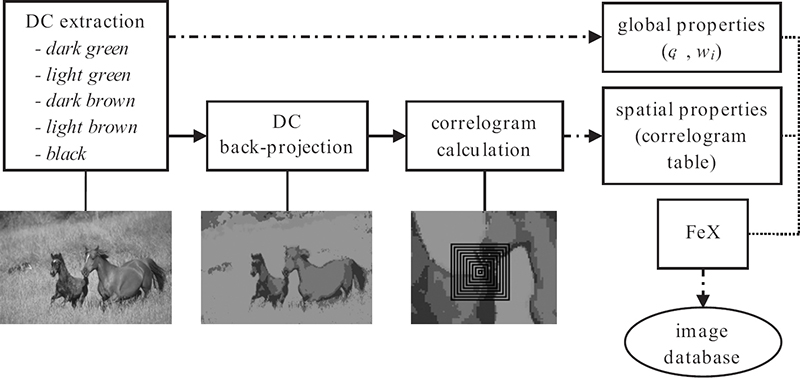
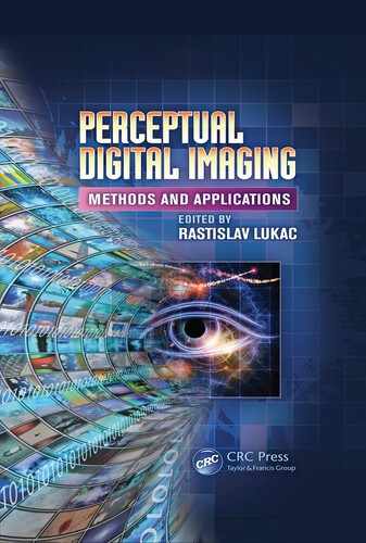
FIGURE 11.3
Overview of the perceptual correlogram descriptor.

11.3 Perceptual Correlogram

In order to obtain the global color properties, DCs are extracted in a way human the visual system perceives them and then back-projected onto the image to extract their spatial relations using the DC-based correlogram. The overview of the feature extraction (indexing) process is illustrated in Figure 11.3. In the retrieval phase, a penalty-trio model is utilized that penalizes both global and spatial dissimilarities in a joint scheme.

11.3.1 Formation of the Color Descriptor

The adopted DC extraction algorithm is similar to one in Reference [33], where the method is entirely designed with respect to human color perception rules and configurable with few thresholds: T_S (color similarity), T_A (minimum area), ε_D (minimum distortion), and $N_{D C}^{\max}$ (maximum number of DCs).

As the first step, the true number of DCs present in the image (that is, $1 \leq N_{D C} \leq N_{D C}^{\max}$ ) are extracted in the CIE-Luv color domain. Let C_i represent the ith DC class (cluster) with the following members: the color value (centroid) c_i and the weight (unit normalized area) w_i. Due to the DC thresholds set beforehand, w_i > T_A and |c_i − c_j| > T_S for 1 ≤ i ≤ N_DC and 1 ≤ j ≤ N_DC. The extracted DCs are then back-projected to the image for further analysis, namely, extraction of the SCD. Spatial distribution of the extracted DCs is represented as a correlogram table as described in Reference [5], except that the colors utilized are the ones coming from the DC extraction; hence, m = N_DC. Thus, for every DC pair on the back-projected image, the probability of finding a pixel with DC c_i at distance of k pixels from a pixel with DC c_j is calculated. The extracted correlogram table and the global features (c_i, w_i) are stored in the database’s feature vector.

11.3.2 Penalty-Trio Model for Perceptual Correlogram

In a retrieval operation in an image database, a particular feature of the query image Q is used for similarity measurement with the same feature of a database image I. Repeating this process for all images in the database D and ranking the images according to their similarity distances yield the retrieval result. In the retrieval phase, while judging the similarity of two image’s global and spatial color properties, two DC lists together with their correlogram tables are to be compared. The more dissimilar colors are present, the larger their similarity distance should be. In order to do so, DCs in both images are subjected to a oneto-one matching. This model penalizes for the mismatching colors together with the global and spatial dissimilarities between the matching through P_φ, which denotes the amount of different (mismatching) DCs, and P_G and P_Corr, which denote, respectively, the differences of the matching DCs in terms of the global differences and correlogram differences.

The overall penalty (color dissimilarity) between query image Q and a database image I over all color properties can be expressed as

$P_{\sum} (Q, I) = P_{ϕ} (Q, I) + (α P_{G} (Q, I) + (1 - α) P_{C o r r} (Q, I)), (11.5)$

where P_∑ ≤ 1 is the (unit) normalized total penalty, which corresponds to (total) color similarity distance, and 0 < α < 1 is the weighting factor between global and spatial color properties of the matching DCs. Thus, the model computes a complete distance measure from all color properties. Note that all global color descriptors mentioned in Section 11.2.1 use only the first two (penalty) terms while discarding P_SCD entirely. The correlogram, on the other hand, works only over P_SCD without considering any global properties. Therefore, the SCD penalty-trio model fuses both approaches to compute a complete distance measure from all color properties. Since color (DC) matching is a key factor in the underlying application, a two-level color partitioning is proposed here. The first level partitions the group of color elements, which are too close for the human eye to distinguish, using a minimum (color) threshold $T_{C}^{\min}$ . Recall from the earlier discussion that such close color elements are clustered into DC classes, that is, |c_i − c_j| ≤ T_S for ∀c_j ∈ C_i, and using the same analogy $T_{C}^{\min}$ can conveniently be set as T_S. Another threshold $T_{C}^{\max}$ is empirically set for second-level partitioning, above which no color similarity can be perceived. Finally, for a given two DCs with the inter-color distance falling between the two levels, that is, $T_{C}^{\min} < | c_{i} - c_{j} | < T_{c}^{\max}$ , there exists a certain level of (color) similarity, but not too close to be perceived as identical.

Define such colors, which show some similarity, as matching, and let $T_{C}^{\max}$ be used to partition the mismatching colors from the matching ones. In order to get a better understanding of the penalty terms, consider a set of matching colors (S^M) and a set of mismatching colors (S^φ) selected among the colors of a database I(C^I) and query Q(C^Q) images, thus S^M + S^Q = C^I + C^Q. Here S^φ consists of the colors that holds |c_i − c_j| > T_S for ∀c_i,c_j ∈ S^φ, and the subset S^M holds the rest of the (matching) colors. Accordingly, P_φ can be defined directly as

$P_{ϕ} (Q, I) = \frac{\sum (w_{i} | c_{i} \in S^{ϕ})}{2} \leq 1. (11.6)$

Consider the case where S^M = {φ}, which means there are no matching colors between images Q and I. Thus P_∑ = P_φ = 1, which makes sense since colorwise there is nothing similar between two images. Conversely, if S^φ = {φ} ⇒ P_φ = 0, the dissimilarity will only emerge from the global and spatial distribution of colors. These distributions are denoted here as P_G and P_Corr, respectively, and can be expressed as follows:

$P_{G} (Q, I) = β \sum_{i = 1}^{N_{M}} | w_{i}^{Q} - w_{i}^{I} | + (1 - β) \frac{1}{T_{S} N_{M}} \sqrt{\sum_{i = 1}^{N_{M}} (c_{i}^{Q} - c_{i}^{I}) 2 \leq 1,} (11.7)$

$P_{C o r r} (Q, I) = \sum_{i, j \in S^{M}} \sum_{k = 1}^{d} {\begin{array}{l} 0 & i f γ_{c_{i}, c_{j}}^{k} (Q) = γ_{c_{i}, c_{j}}^{k} (I) = 0 \\ \frac{| γ_{c_{i}, c_{j}}^{(k)} (Q) - γ_{c_{i}, c_{j}}^{(k)} (I) |}{γ_{c_{i}, c_{j}}^{(k)} (Q) + γ_{c_{i}, c_{j}}^{(k)} (I)} & o t h e r w i s e \end{array}}, (11.8)$

where $γ_{c_{i}, c_{j}}^{(k)}$ is the probability of finding DC c_i at a distance k from DC c_j, and 0 < β < 1 in P_G provides the adjustment between color area (weight) difference indicated by the first term and DC (centroid) difference of the matching colors indicated by the second term. Note that the distance function used for comparing two correlogram tables (P_Corr) differs from the formulation proposed in Reference [5], which avoids divisions by zero by adding the value of one to the denominator. However, correlogram values are the probabilities that hold 0 < $γ_{c_{i}, c_{j}}^{(k)}$ < 1, thus such an addition becomes relatively significant and introduces a bias to distances; hence, it is strictly avoided in proposed distance calculations. As a result, the weighted combination of P_G and P_Corr represents the amount of dissimilarity that occurs in the color properties; through the weight α one color property can be favored over another. With the combination of P_φ, the penalty trio models a complete similarity distance metric between two color compositions.

11.3.3 Retrieval Performance on Synthetic Images

The perceptual correlogram and the two traditional descriptors, that is, correlogram and MPEG-7 dominant color descriptor (DCD), are implemented as a feature extraction (FeX) module within MUVIS framework [11] in order to test and perform performance comparisons in the context of CBIR. All descriptors are tested using two separate databases on a personal computer with 2 GB of RAM and Pentium 4 central processing unit (CPU) operating at 3.2 GHz.

First database has 1088 synthetic images that are formed of arbitrary shaped and colored regions. In this way, the color matching accuracy can visually be tested and the penalty terms P_φ, P_G, and P_Corr can individually be analyzed via changing the shape and/or size of any color regions. Furthermore, the robustness against resolution, translation, and rotation changes can be compared against the traditional correlogram. First, twelve retrievals of two queries from the synthetic database are shown in Figure 11.4. In Q1, correlogram’s area insensitivity, due to its probabilistic nature, can clearly be observed. It can retrieve the first relevant image only at the eight rank, whereas the perceptual correlogram retrieves seven similar color compositions on the first page using d = 10 and still fails to bring them to higher ranks due to the limited range value (d = 10). For d = 40, all relevant images sharing with similar color compositions can be retrieved in the highest ranks. In the same figure, Q2 demonstrates the resolution dependency of the correlogram, which fails to retrieve the image with identical color structure but different resolution in the first page. Even though the penalty-trio model aids to overcome the resolution dependence problem, note that this descriptor still utilizes the correlogram as the spatial descriptor and hence the perceptual correlogram manages to retrieve it only at the third rank and despite severe resolution differences, it can further retrieve most of the relevant images on the first page.

Images

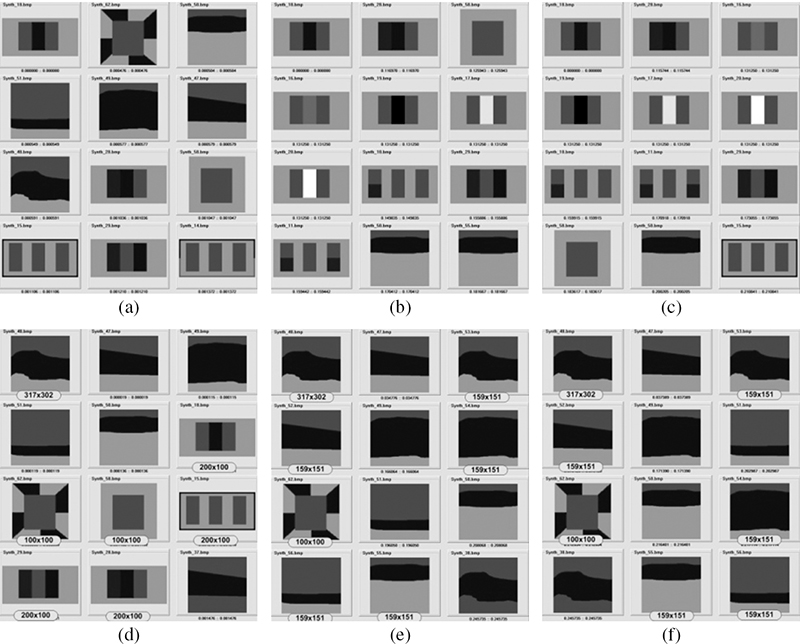
FIGURE 11.4
Two queries Q1 (a–c) and Q2 (d–f) in the synthetic database with typical and perceptual correlograms with different parameters: (a,d) typical correlogram, (b,e) perceptual correlogram for d = 10, and (c,f) perceptual correlogram for d = 40. Top-left is the query image.

11.3.4 Retrieval Performance on Natural Image Databases

The second database has 10000 medium resolution (384 × 256 pixels) images from diverse contents selected from the Corel image collection. The recommended distance metrics are implemented for each FeX module, that is the quadratic distance for MPEG-7 DCD and L₁ norm for the correlogram. Due to its memory requirements, the correlogram could be implemented only with m = 27 colors (3 × 3 × 3 bins RGB histogram) and d = 10, since further increase in either setting is infeasible in terms of computational complexity. In order to measure the retrieval performance, an unbiased and limited formulation of normalized modified retrieval rank NMRR (q) is used here, which is defined in MPEG-7 as the retrieval performance criteria per query q. It combines both of the traditional hit-miss counters; Precision –Recall, and further takes the ranking information into account as follows:

Images

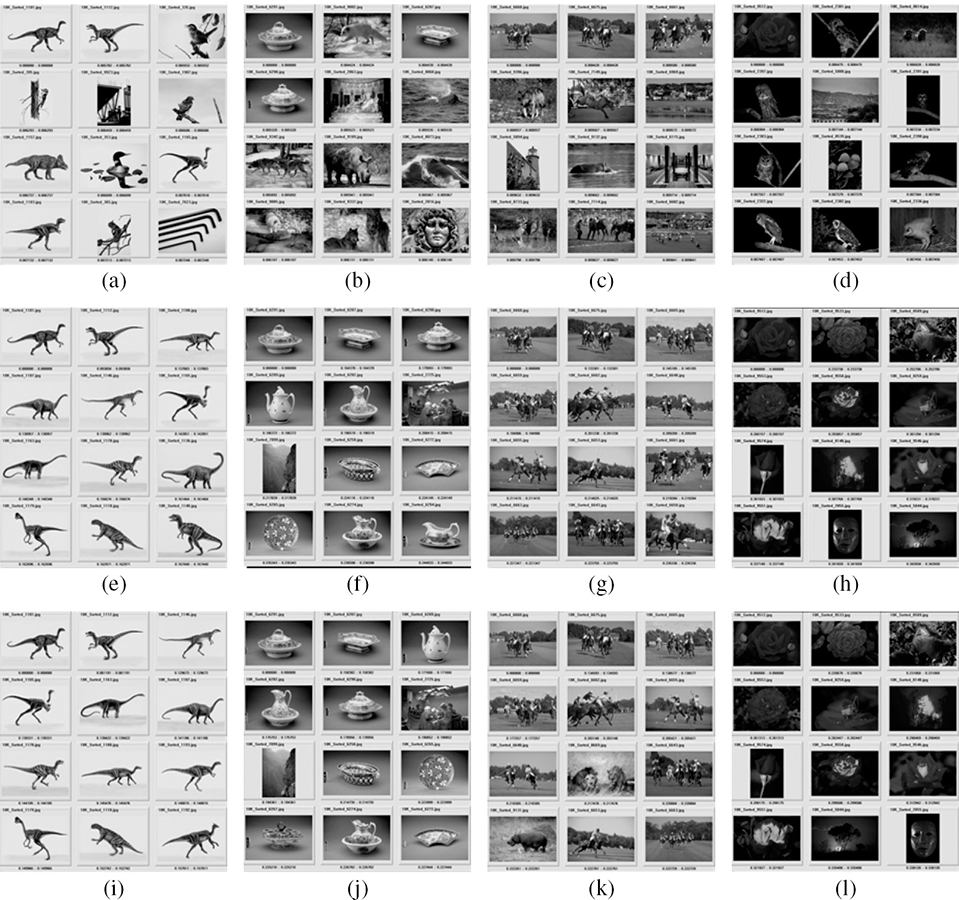
FIGURE 11.5 (See color insert.)
Four queries in Corel 10K database: (a–d) correlogram for d = 10, (e–h) perceptual correlogram for d = 10, and (i–l) perceptual correlogram for d = 40. Top-left is the query image.

$A V R (q) = \frac{1}{N (q)} \sum_{N (q)}^{N (q)} R (k) w i t h W = 2 N (q), (11.9)$

$N M R P (q) = \frac{2 A V R (q) - N (q) - 1}{2 W - N (q) + 1} \leq 1, (11.10)$

$A N M R R = \frac{1}{Q} \sum_{q = 1}^{Q} N M R R (q) \leq 1, (11.11)$

TABLE 11.1
ANMRR results for Corel 10K database.

Method	Score
MPEG7 DCD	0.495
correlogram for d = 10	0.422
perceptual correlogram for d = 10	0.391
perceptual correlogram for d = 40	0.401

where N(q) is the minimum number of relevant images (based on ground-truth) in a set of Q retrieval experiments, R(k) is the rank of the kth relevant retrieval within a window of W retrievals, which are taken into consideration during per query q. If there are less than N(q) relevant retrievals among W, then a rank of W + 1 is assigned for the remaining ones. The term AV R(q) is the average rank obtained from the query q. Since each query item is selected within the database, the first retrieval will always be the item queried and this obviously yields a biased NMRR (q) calculation; therefore, it is excluded from ranking. Hence, the first relevant retrieval R (1) is ranked by counting the number of irrelevant images a priori and if all N(q) retrievals are relevant, then NMRR(q) = 0; the best retrieval performance is thus achieved. On the other hand, if none of relevant items can be retrieved among W, then NMRR(q) = 1 as the worst case. Therefore, the lower NMRR(q), the better (more relevant) the retrieval is for the query q. Keeping the number of query-by-example experiments sufficiently high, the average NMRR and ANMRR can thus be used as the retrieval performance criteria.

In total, 104 query-by-example experiments were performed for each descriptor, with some retrieval results shown in Figure 11.5. The average scores are listed in Table 11.1.

The perceptual correlogram extracts both global and spatial color properties throughout the whole image, thus erroneous queries such as in Figure 11.2 can be avoided where global color properties vary significantly (for example, see Figure 11.6).

Images

FIGURE 11.6 (See color insert.)
Retrieval result of the perceptual correlogram for the query in Figure 11.2.

Images

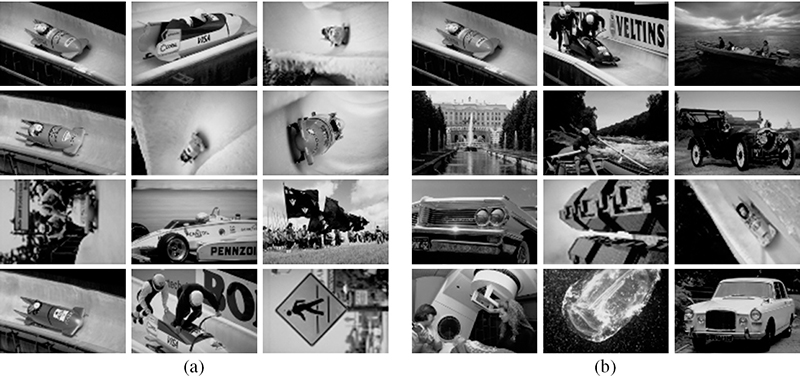
FIGURE 11.7 (See color insert.)
A special case where the correlogram works better than the perceptual correlogram descriptor: (a) correlogram and (b) perceptual correlogram.

As discussed earlier, in some particular cases, the traditional correlogram may yield a better retrieval performance than the perceptual correlogram. Figure 11.7 shows a typical example, where the images retrieved using the correlogram are the zoomed versions of the query image or they are all taken from different viewpoints. Apart from such special query examples, the perceptual correlogram achieved better retrieval performance on the majority of the queries performed. Yet the most important point is the feasibility issue of both descriptors. Note that the utilization of the traditional correlogram is only possible because image resolution is fairly low (384 × 256 pixels), database contains only 10000 images, and the range value d is quite limited (d = 10). Even with such settings, the correlogram required 556 MB disk space and 850 MB memory (fast algorithm) during the feature extraction phase, whereas the perceptual correlogram takes 53 MB disk space and 250 MB memory for $N_{D C}^{\max}$ = 8 and d = 10, thus reducing the storage space by approximately 90% and the computational memory (fast algorithm) by 70%. Henceforth, only the perceptual correlogram descriptor can be used if a further increase occurs in any of the settings.

11.4 Spatial Color Descriptor

Under the light of the earlier discussion, an efficient spatial color descriptor (SCD) is designed to address the drawbacks and problems of the color descriptors, particularly the color correlogram. In order to achieve this goal, various perception rules are followed by extracting and describing the global and spatial color properties in a way as perceived by the HVS. Namely, outliers in color and spatial domains are suppressed or eliminated by adopting a top-down approach during feature extraction. The SCD is formed by a proper combination of global and spatial color features. During the retrieval phase, the similarity between two images is computed using a penalty-trio model, which penalizes the individual differences in global and spatial color properties. In the following subsections, both indexing (feature extraction) and retrieval schemes are discussed in detail.

11.4.1 Formation of the Spatial Color Descriptor

As previously discussed, the DCs represent the prominent colors in an image while the imperceivable color components (outliers) are discarded. As a result, they have a global representation, which is compact and accurate, and they represent few dominant colors that are present and perceivable in an image. For a color cluster C_i, its centroid c_i is given by

$c_{i} = \frac{\sum w (p) x (p)}{\sum w (p)}, f o r x (p) \in C_{i}, (11.12)$

and the initial clusters are determined by using a weighted distortion measure, defined as

$D_{i} = \sum w (p) {‖ x (p) - c_{i} ‖}^{2}, f o r x (p) \in C_{i} . (11.13)$

These definitions are used to determine which clusters to split until either $N_{D C}^{\max}$ denoting a maximum number of clusters (DCs) is achieved or ε_D denoting a maximum allowed distortion criteria is met. Hence, pixels with smaller weights (detailed sections) are assigned to fewer clusters so that the number of color clusters in the detailed regions, where the likelihood of outliers’ presence is high, is suppressed. As the final step, an agglomerative clustering (AC) is performed on the cluster centroids to further merge similar color clusters so that there is only one cluster (DC) hosting all similar color components in the image. A similarity threshold T_S is assigned to the maximum color distance possible between two similar colors in a certain color domain (for instance, CIE-Luv, CIE-Lab). Another merging criterion is the color area, that is, any cluster should have a minimum amount of coverage area T_A so as to be assigned as a DC; otherwise, it will be merged with the closest color cluster since it is just an outlier. Another important issue is the choice of the color space since a proper color clustering scheme for DC extraction tightly relies on the metric. Therefore, a perceptually uniform color space should be used and the most common ones are CIE-Luv and CIE-Lab, which are designed such that perceived color distances are qual for the Euclidean (L₂) distance in these spaces. The HSV space, although it represents an intuitive color domain, suffers from discontinuities and the RGB color space is not perceptually uniform. To this end, among CIE-Luv and CIE-Lab, the former one is selected here since it yields a lower transformation cost from native RGB space. For CIE-Luv, a typical value for T_S is between 10 and 20, whereas T_A is between 2 to 5% [28], and ε_D< 0.05. Based on the earlier remarks, $N_{D C}^{\max}$ can be conveniently set to 8. As shown in Figure 11.8, the employed DC extraction method is similar to the one in Reference [33], which is entirely designed with respect to HVS color perception rules and configurable with few thresholds, T_S (color similarity), T_A (minimum area), ε_D (minimum distortion), and $N_{D C}^{\max}$ (maximum number of DCs). As the first step, the true number of DCs present in the image (that is, $1 \leq N_{D C} \leq N_{D C}^{\max}$ ) is extracted in CIE-Luv color domain and back-projected to the image for further analysis involving extraction of the spatial properties (SCD) of DCs. Let C_i represents the ith DC class (cluster) with the following members: c_i is the color value (centroid), w_i is the weight (unit normalized area), and σ_i is the standard deviation obtained from the distribution of (real) colors clustered by C_i. Due to the DC thresholds set beforehand, w_i > T_A and |c_i − c_j| > T_S for 1 ≤ i ≤ N_DC and 1 ≤ j ≤ N_DC.

During the back-projection phase, the DC with the closest centroid value to a particular pixel color will be assigned to that pixel. As a natural consequence of this process, spatial outliers, that is, isolated pixel(s), which are not populated enough to be perceivable, can emerge (see Figure 11.8) and should thus be eliminated. Due to the perceptual approach based on the Gestalt rule that states “humans see the whole before its parts,” a top-down approach, such as quad-tree decomposition, can process the whole first, meaning the largest blocks possible which can be described (and perceived) by a single DC, before going into its parts. Due to its top-down structure, the SCD scheme does not suffer from the aforementioned problems of some pixel-based approaches.

Two parameters are used to configure the quad-tree (QT): T_W, which is the minimum weight (dominance) within the current block required from a DC not to go down for further partition and $D_{Q T}^{\max}$ , which is the depth limit indicating the maximum amount of partition (decomposition) allowed. Note that with the proper setting of T_W and $D_{Q T}^{\max}$ , QT decomposition can be carried out to reach the pixel level; however, such an extreme partitioning should not be permitted to avoid the aforementioned problems of pixel-level analysis. Using a similar analogy, T_W can be set in accordance with T_A, that is, T_W ≅ = 1 − T_A. Therefore, for the typical T_A setting (between 2 and 5%), T_W can be conveniently set as T_W ≥ 95%. Since $D_{Q T}^{\max}$ determines when to stop the partitioning abruptly, it should not be set too low so that it does not cause inhomogeneous (mixed) blocks. On the other hand, extensive experimental results suggest that $D_{Q T}^{\max}$ > 6 is not required even for the most complex scenes since the results are almost identical to the one with $D_{Q T}^{\max}$ = 6. Therefore, the typical range is $4 \leq D_{Q T}^{\max} \leq 6$ . Let B^p corresponds to the pth partition of the block B, where p = 0 is the entire block and 1 ≤ p ≤ 4 represents the pth quadrant of the block. The four quadrants can be obtained simply by applying equal partitioning to the parent block or via any other partitioning scheme, which can be optimized to yield most homogenous blocks possible. For simplicity the former case is used here, and accordingly a generic QT algorithm can be expressed as depicted in Algorithm 11.1.

ALGORITHM 11.1 QuadTree(parent, depth).

Let w_max be the weight of the DC which has the minimum coverage in parent block.
If w_max > T_w, then return.
Let B₀ = parent.
For ∀ p ∈ [1,2,3,4] do QuadTree(B^p, depth).
Return.

The QT decomposition of a (back-projected) image I can then be initiated by calling QuadTree(I,0) and once the process is over, each QT block carries the following data: its depth $D \leq D_{Q T}^{\max}$ where the partitioning is stopped, its location in the image, the major DC with the highest weight in the block (that is, w_max > T_W), and perhaps some other DCs which are eventually some spatial outliers. In order to remove those spatial outliers, a QT back-projection of the major DC into its host block is sufficient. Figure 11.8 illustrates the removal of some spatial outliers via QT back-projection on a sample image. The final scheme, where outliers in both color and spatial domains are removed and the (major) DCs are assigned (back-projected) to their blocks, can be conveniently used for further (SCD) analysis to extract spatial color features. Note that QT blocks can vary in size depending on the depth, yet even the smallest (highest depth) block is large enough to be perceivable, and carry a homogenous DC. So instead of performing pixel-level analysis, such as in the correlogram, the uniform grid of blocks in the highest depth ( $D = D_{Q T}^{\max}$ ) can be used for characterizing the global SCD and extracting the spatial features in an efficient way. As shown in Figure 11.8, one of the two modes, which perform two different approaches to extract spatial color features, can be used. The first is the scalar mode, over which inter-DC proximity histograms are computed within the full image range. These histograms indicate the amount of a particular DC that can be found from a certain distance of another DC; however, this is a scalar measure which lacks the direction information. For example, such a measure can state “17% of red is eight units (blocks) away from blue,” which does not provide any directional information. Therefore, the second mode is designed to represent inter-occurrence of one DC with respect to another over a two-dimensional (proximity) grid, from which both distance and direction information can be obtained. Note that inter-color distances are crucial for characterizing the SCD of an image; however, the direction information may or may not be useful depending on the content. For example, the direction information in “17% of red is eight units (blocks) right of blue” is important for describing a national flag and hence the content, but “one black and one white horse are running together on a green field” is sufficient to describe the content without any need to know the exact directional order of black, white, and green. The following subsections will first detail both modes and then evaluate their computational and retrieval performances individually.

Images

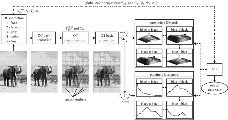
FIGURE 11.8
Overview of the SCD formation.

11.4.2 Proximity Histograms-Based Description

Once the QT back-projection of major DCs into their host blocks are completed, all QT blocks hosting a single (major) DC with a certain depth ( $D \leq D_{Q T}^{\max}$ ) are further partitioned into the blocks in highest depth ( $D = D_{Q T}^{\max}$ ) to achieve a proximity histogram in the highest blockwise resolution. Therefore, in such a uniform block-grid, the image I will have N × N blocks for $N = 2^{D_{Q T}^{\max}}$ , each of which hosts a single DC. Accordingly the problem of computing inter-DC proximities turns out to be block distances and hence the block indices in each dimension (that is, ∀x,y ∈ [1, N]) can directly be used for distance (proximity) calculation. Since the number of blocks does not change with respect to image dimension(s), resolution invariance is achieved (for example, the same image in different resolutions will have identical proximity histograms/grids as opposed to significantly varying correlograms due to its pixel-based computations). As shown in Figure 11.8, one can use either L₁ or L_∞ norms for block-distance calculations. Let b₁ = (x₁, y₁) and b₂ = (x₂,y₂) be two blocks, their distance for the L₁ norm can be defined as ‖b₁ − b₂‖ = |x₁ − x₂| + |y1 − y₂|, and for the L_∞ norm as ‖b₁ − b₂‖ = max(|x₁ − x₂|, |y₁ − y₂|), respectively. Using the block indices in both norms, the block distances become integer numbers and note that for a full range histogram, the maximum (distance) range will be [1,L], where L is N − 1 in L_∞ and 2N − 2 in L₁ norms, respectively. A blockwise proximity histogram for a DC pair c_i and c_j stores in its kth bin the number of blocks hosting c_j (that is, ∀b_j ‖I(b_j) = c_j, equivalent to the amount of color c_j in I) from all blocks hosting c_i (that is, ∀b_i|I(b_i) = c_i, equivalent to amount of color c_i in I) at a distance k. Such a histogram clearly indicates how close or far two DCs and their spatial distribution with respect to each other are. Yet the histogram bins should be normalized by the total number of blocks, which can be found k blocks away from the source block b_i hosting the DC c_i, because this number will significantly vary with respect to the distance (k), the position of source block (b_i), and the norm (L₁ or L_∞) used. Therefore, the kth bin $Φ_{c_{i}}^{c_{j}} (k)$ of the normalized proximity histogram between the DC pair c_i and cj can be expressed as follows:

Images

FIGURE 11.9
N(b_i,k) templates in 8 × 8 block grid ( $D_{Q T}^{\max}$ = 3) for three range values in L_∞ (top) and L₁ (bottom) norms.

$Φ_{c_{i}}^{c_{j}} (k) \sum_{b_{i}} \sum_{b_{j}} Δ (b_{i}, b_{j}, k), (11.14)$

where

$Δ (b_{i}, b_{j}, k) = {\begin{array}{l} N {(b_{i}, k)}^{- 1} & i f b_{i} \in I (c_{i}), b_{j} \in I (c_{j}), ‖ b_{i} - b_{j} ‖ = k, \\ 0 & o t h e r w i s e . \end{array} (11.15)$

The normalization factor N(b_i, k), denoted as the total number of neighbor blocks in distance k, is independent from the DC distribution and hence it is only computed once and used for all images in the database. Figure 11.9 shows N(b_i, k) templates computed for all blocks (∀b_i ∈ I), both norms, and some range values. In this figure, N is set to eight ( $D_{Q T}^{\max}$ = 3) for illustration purposes. Note that normalization cannot be applied for blocks with N(b_i, k) = 0, since k is out of image boundaries and hence $Φ_{c_{i}}^{c_{j}} (k)$ = 0 for ∀c_i.

Once the N(b_i,k) templates are formed, computing the normalized proximity histogram takes O(N⁴). Note that this is basically independent from the image dimensions W and H, and it is also a full-range computation (that is, k ∈ [1, L]), which may not be necessary in general (say, half image range may be quite sufficient since above this range most of the central blocks will have either out-of-boundary case, where $Φ_{c_{i}}^{c_{j}} (k) = 0 f o r \forall c_{i}$ , or only few blocks are within the range, which is too low for obtaining useful statistics). A typical setting $D_{Q T}^{\max}$ = 5, which implies N = 32 and $N = 32 a n d N_{D C}^{\max}$ = 8, requires O(10⁶) computations, which is 10000 times less compared to the correlogram with a minimal range setting (10% of image dimension range). In fact, the real speed enhancement is much more since the computations in the correlogram involve several additions, multiplications, and divisions (worst of all) for probability computations, whereas only additions are sufficient for computing $Φ_{c_{i}}^{c_{j}} (k)$ as long as N(b_i,k)⁻¹ is initially computed and stored as the template. The memory requirements for the full-range computation are O(N²L) for storing N(b_i,k)⁻¹ and plus $O (N_{D C}^{2} L)$ for computing $Φ_{c_{i}}^{c_{j}} (k)$ , respectively. The memory space required for the typical settings given earlier will thus be 500 Kb, which is a significant reduction compared to that of the correlogram. The typical storage space required per database image is less than 17 Kb with L_∞, and less than 33 Kb with L₁ norm, which is eventually 50 times smaller than the auto-correlogram’s requirement O(md) with minimal m and d settings.

Images

FIGURE 11.10
The process of proximity grid formation for the block (X) for L=4.

11.4.3 Two-Dimensional Proximity Grids-Based Description

An alternative approach for characterizing the inter-DC distribution uses the respective proximities and also their inter-occurrences accumulated over a two-dimensional proximity grid. The process starts from the same configuration outlined earlier. Let the image I have N × N blocks, each of which hosts a single DC. The two-dimensional proximity grid, $Ψ_{c_{i}}^{c_{j}} (x, y)$ , is formed by cumulating the co-occurrence of blocks hosting c_j (that is, ∀b_j‖I(b_j) = c_j) in a certain vicinity of the blocks hosting c_i (that is, ∀b_i|I(b_i) = c_i) over a two-dimensional proximity grid. In other words, by fixing the block b_i (hosting c_i) in the center bin of the grid (x = y = 0), the particular bin corresponding to the relative position of block b_j (hosting c_j) is incremented by one and this process is repeated for all blocks hosting c_j in a certain vicinity of b_i. Then, the process is repeated for the next block (hosting c_i) until the entire image blocks are scanned for the color pair (c_i,c_j). As a result, the final grid bins represent the inter-occurrences of the cj blocks with respect to the ones hosting color c_i within a certain range L (that is, ∀x,y ∈ [−L,L], with L ≤ N − 1). Although L can be set as N − 1 for a full-range representation, this is a highly redundant setting since L ≤ N/2 cannot be fit exactly for any block without exceeding the image (block) boundaries. Therefore, L < N/2 would be a reasonable choice for L.

Images

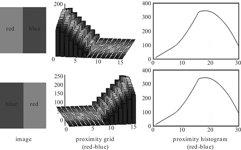
FIGURE 11.11
Proximity grid compared against histogram for a sample red-blue color pair.

The computation of $Ψ_{c_{i}}^{c_{j}} (x, y)$ can be performed in a single pass through all image blocks. Let b_i(x_i, y_i) be the next block hosting the DC c_i. Fixing b_i in the center (that is, $Ψ_{c_{i}}^{c_{j}} (0, 0)$ ), all image blocks within the range L from b_i (that is, ∀b_j = (x_i + x, y_i + y)∈ I | ∀x,y ∈ [−L, L]) are scanned and the corresponding (proximity) grid bin $Ψ_{c_{i}}^{c_{j}} (x, y)$ for a color c_j in a block b_j = (x_i + x, y_i + y)∈ I is incremented by one. This process is illustrated on a sample image shown in Figure 11.10. During the raster-scan of uniform blocks, the block with white DC updates only three proximity grids (white to white, brown, and blue), since those DCs can only be found within the range of ±L. For illustration purposes, $D_{Q T}^{\max}$ = 5 which implies N = 32, and L = 4. As a result, such a proximity grid characterizes both inter-DC proximities and the relative spatial position (inter-DC direction) between two DCs. This is straightforward to see in the sample images in Figure 11.11, where the proximity grid distinguishes the relative direction of a DC pair (red-blue), while the proximity histogram cannot do it due to its scalar metric. Note that $Ψ_{c_{i}}^{c_{j}} (0, 0)$ = 0 for i ≠ j, and $Ψ_{c_{i}}^{c_{j}} (0, 0)$ indicates the total number of blocks hosting c_i. Since this is not a SCD property, rather a local DC property showing a noisy approximation of w_i (weight of c_i), it can be conveniently excluded from the feature vector and the remaining (2L + 1)²− 1 grid bins are (unit) normalized by the total number of blocks N² to form the final descriptor ${\bar{Ψ}}_{c_{i}}^{c_{j}} (x, y)$ , where ${\bar{Ψ}}_{c_{i}}^{c_{j}} (x, y) \leq 1 f o r \forall x, y \in [- L, L]$ .

The proximity grid computation takes O(N²L²). Similar to the proximity histogram, this is also independent from original image dimensions W and H, and for a full-range process (L = N/2), the same number of computations equal to O(N⁴) is obtained. However, instead of regular addition operations required for the proximity histogram, or multiplications and divisions for the correlogram, the proximity grid computation requires only incrementing operations. Thus, for a typical grid dimension range, for example, N /8 < L < N /4, computing the proximity grid takes the shortest time. The memory space requirement is in $O (N_{D C}^{2} L^{2})$ and for a full-range process (L = N /2) with the typical settings $D_{Q T}^{\max}$ = 5 implying N = 32, and $N_{D C}^{\max}$ = 8, the memory required per database image will be 256 Kb. This is still smaller than O(md) by the auto-correlogram even with the minimal m and d settings, and it is equivalent to half of the memory required for the proximity histogram. Since $Ψ_{c_{i}}^{c_{j}} (x, y) = Ψ_{c_{j}}^{c_{i}} (- x, - y)$ , which indicates the symmetry with respect to origin, the storage (disk) space requirement is even less, namely, $O (N_{D C}^{2} L^{2})$ . However, it requires eight times more space than the proximity histogram. This is the cost of computing full-range proximity grid, and therefore, it is recommended to employ the typical grid dimension range (for example, N / 8 < L < N /4) to reduce this cost to an acceptable level.

11.4.4 Penalty-Trio Model for Spatial Color Descriptors

As previously discussed, the penalty-trio model used therein provides a balanced similarity metric that encapsulates three crucial global and spatial color properties. Therefore, a similar penalty-trio model is adopted for computing the similarity distance between two SCDs. As shown in Figure 11.8, the SCDs of Q and I contain both global and spatial color properties. Let $C_{i}^{Q} a n d C_{j}^{I}$ represent the ith and jth $(i \leq N_{D C}^{Q}, j \leq N_{D C}^{I})$ DC classes, where $N_{D C}^{Q} a n d N_{D C}^{I}$ are the number of DCs in Q and I, respectively. Along with these global properties, the SCD descriptors of Q and I contain either proximity histogram $Ψ_{c_{i}}^{c_{j}} (k)$ or grid $Ψ_{c_{i}}^{c_{j}} (x, y)$ depending on the SCD mode. Henceforth, for the similarity distance computation over the SCD, both global and spatial color properties are used within a similar penalty-trio model used earlier, which basically penalizes the mismatches between Q and I. The three mismatches considered here are P_φ denoting the amount of different DCs, and the differences of the matching DCs in global color properties expressed via P_G and SCD properties expressed via P_SCD. Thus, the penalty-trio over all color properties can be expressed as

$P_{\sum} (Q, I) = P_{ϕ} (Q, I) + (α P_{G} (Q, I) + (1 - α) P_{S C D} (Q, I)), (11.16)$

where P_∑≤ 1 is the normalized total penalty, which corresponds to the total color similarity distance, and 0< α< 1 is the weighting factor between global and spatial color properties.

As mentioned earlier, one can form two sets, that is, matching (S^M) and mismatching (S^φ) DC classes from C^Q and C^I. This is accomplished by assigning each DC c_i ∈ C_i in one set, which cannot match any DC c_j ∈ C_j in the other (implying |c_i − c_j| > $T_{C}^{\max}$ for all i and j) into S^Φ and the rest (with at least one match) into S^M. Note that S^M + S^Φ = C^Q + C^I, and using the DCs in S^Φ, the term P_Φ can directly be expressed as given in Equation 11.6. Recall that the dissimilarity (penalty P_φ) increases proportionally with the total amount (weight) of mismatching DCs. In one extreme case, where there are no colors matching, S^M = {φ} implying P_∑ = P_φ = 1 means that the two images have no similar (matching) colors. In another extreme case, where all DCs are matching, so S^φ = {φ} implying P_φ = 0, color similarity will only emerge from global P_G and spatial P_SCD color properties of the (matching) DCs. Typically, P_φ contributes a certain color distance as a natural consequence of mismatching colors between Q and I, yet the rest of the distance will result from the cumulated difference of color matching. This is, however, not straightforward to compute since one DC in Q can match one or more DCs in I (or vice versa). One solution is to apply color quadratic distance [12] to fuse DC distances into the total similarity metric. However, besides its serious drawbacks mentioned earlier, this formulation can be applied only to distance calculation from global DC properties and hence cannot address the problem of fusing SCD distances (from proximity grid or histogram of each individual DC pair). Another alternative is to enforce a one-to-one DC matching, that is, one DC alone in Q can match a single DC in I by choosing the best match and discarding the other matches. This, as well, induces serious errors due to the fact that DC extraction is a dynamic clustering algorithm in color domain and due to variations in color composition of the scenery or its predetermined parameters (thresholds), it can result in over-clustering or under-clustering. Therefore, similar color compositions can be clustered into different number of DCs and enforcing one-to-one matching may miss part of matching DCs from both global and spatial similarity computation.

Images

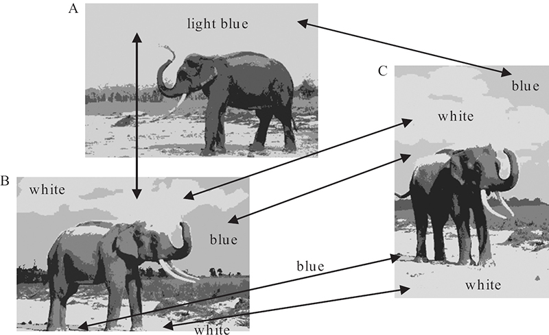
FIGURE 11.12
One-to-one matching of DC pairs among three images.

A typical example of such a consequence can be seen in Figure 11.12 which shows three images with highly similar content, that is, “an elephant under cloudy sky.” In two images (B and C), the cloud and sky are distinguished during DC extraction with separate blue and white DCs; however, in image A, only one DC (light blue) is extracted with the same parameters. Consequently, there is no (one-to-one) matching problem between B and C and such a matching will naturally reflect similar global and spatial DC properties. However, between A and B or C, if the single DC (light blue) is matched only with one DC (white or blue), this will obviously yield an erroneous result on both global and spatial similarity computations since neither DC (white or blue) properties such as weight, distribution, and proximities to other DCs are similar to the one in A (light-blue).

As a result, before computing P_G and P_SCD, the DC sets in Q (or I), which are in a close vicinity of a single DC in I (or Q) should be first fused into a single DC. For instance, in Figure 11.12, the DC light-blue in image A is close to both white and blue in image B (and C); therefore, both colors in B should be fused into a new DC (perhaps a similar light-blue color) and then P_G and P_SCD can be computed accurately between A and B. In order to accomplish this, $T_{C}^{\min} = T_{S}$ is used for matching the close DCs and a twofold matching process is performed via function TargetMatch, which first verifies and then fuses some DCs in the target set T, if required by any DC in the source set S. Let $S_{Q}^{M} \subset S^{M} a n d S_{I}^{M} \subset S^{M}$ be the sets of matching DCs for Q and I, respectively. Since any DC in any set can request fusing two or more DCs in the other set, the function is called twice, that is, first $T \arg e t M a t c h (S_{Q}^{M}, S_{I}^{M})$ and then $T \arg e t M a t c h (S_{I}^{M}, S_{Q}^{M})$ . Accordingly, TargetMatch can be expressed as depicted in Algorithm 11.2.

ALGORITHM 11.2 TargetMatch(S, T).

For ∀c_i∈ S, let $L_{i}^{M}$ be the matching DC list for c_i.
For ∀c_j ∈ T, if |c_i − c_j| ≤ T_S, then c_j → $L_{i}^{M}$ .
If $| L_{i}^{M} | \geq 2$ then:
- Let $L_{i}^{N} = T - L_{i}^{M}$ be the non-matching list.
- $C_{x} = F u s e D C s (L_{i}^{M}, L_{i}^{N})$
- Update $T = L_{i}^{N} + C_{x}$ .
Return.

ALGORITHM 11.3 FuseDCs $(L_{i}^{M}, L_{i}^{N})$ .

Create C_x: {c_x,w_w,s_x} by fusing $\forall c_{j} \in L_{i}^{M}$ .
- $w_{x} = \sum_{C_{j} \in L_{i}^{M}} w_{j}$
- $c_{x} = \frac{\sum_{C_{j} \in L_{i}^{M}} w_{j} c_{j}}{\sum_{C_{j} \in L_{i}^{M}} w_{j}} a n d \frac{\sum_{C_{j} \in L_{i}^{M}} w_{j} σ_{j}}{\sum_{C_{j \in L_{i}^{M}}} w_{j}}$
Form both $X_{c_{x}}^{c_{x}} a n d (X_{c_{x}}^{c_{j}} - X_{c_{j}}^{c_{x}}) | \forall c_{j} \in L_{i}^{N}$ .
- $X_{c_{x}}^{c_{x}} = \sum_{C_{j} \in L_{i}^{M}} \sum_{C_{k} \in L_{i}^{M}} X_{c_{j}}^{c_{k}}$
- $X_{c_{x}}^{c_{j}} = \sum_{C_{k} \in L_{i}^{M}} X_{c_{j}}^{c_{k}} | \forall_{c_{j}} \in L_{i}^{N}$
- Compute $X_{c_{j}}^{c_{j}} f r o m X_{c_{j}}^{c_{x}}, \forall c_{j} \in L_{i}^{N}$ .
Return C_x.

The function FuseDCs depicted in Algorithm 11.3 fuses all DCs in the list $L_{i}^{M}$ , reforms the SCD descriptors of all (updated) DC pairs $Ψ_{c_{i}}^{c_{j}} (k) o r Ψ_{c_{i}}^{c_{j}} (k)$ , and finally returns a new (fused) DC C_X. Then, the target set T is updated accordingly. Let $X_{c_{i}}^{c_{j}}$ be the SCD operator (that is, $Φ_{c_{i}}^{c_{j}} o r Ψ_{c_{i}}^{c_{j}}$ depending on the SCD mode as shown in Figure 11.8) and $X_{c_{j}}^{c_{1}} + X_{c_{i}}^{c_{2}}$ be defined as

$X_{c_{i}}^{c_{1}} + X_{c_{i}}^{c_{2}} = {\begin{array}{l} Φ_{c_{i}}^{c_{1}} (k) + Φ_{c_{i}}^{c_{2}} (k) & f o r \forall k \in [1, L] \\ Ψ_{c_{i}}^{c_{1}} (x, y) + Ψ_{c_{i}}^{c_{2}} (x, y) & f o r \forall x, y \in [- L, L] \end{array} (11.17)$

Furthermore, let ⊕ be the fusing operator over DC classes. It is simple to show that $X_{c_{i}}^{c_{1} \oplus c_{2}} = X_{c_{i}}^{c_{1}} f o r c_{1, 2} \neq c_{i}$ . Once the DCs in $L_{i}^{M}$ are fused, they are removed along with their SCD descriptors while keeping the DCs (and their internal SCD descriptors) in $L_{i}^{N}$ intact. The new (fused) DC C_X (along with its SCD descriptors) is inserted into the target set T. Recall from the earlier remarks on SCD descriptor properties that $Φ_{c_{i}}^{c_{j}} (k) = Φ_{c_{j}}^{c_{i}} (k)$ and $Ψ_{c_{i}}^{c_{j}} (x, y) = Ψ_{c_{j}}^{c_{i}} (- x, - y)$ ; therefore, once $X_{c_{j}}^{c_{x}} f o r \forall c_{j} \in L_{i}^{N}$ are formed, it is straightforward to compute $X_{c_{x}}^{c_{j}} f o r \forall c_{j} \in L_{i}^{N}$ . After the consecutive calls of TargetMatch function, all DC sets in each set, which are close (matching) to a particular DC in the other set, are fused. Thus, one-to-one matching can be conveniently performed by selecting the best matching pair in both sets. As a result, the number of DCs in both (updated) sets $S_{Q}^{M} a n d S_{I}^{M}$ becomes equal, that is, $| S_{Q}^{M} | = | S_{I}^{M} | = N_{M}$ . Assume without loss of generality that ith DC class in set $C_{i}^{Q} : {c_{i}^{Q}, w_{i}^{Q}, σ_{i}^{Q}} \in S_{Q}^{M}$ matches the ith DC in set $C_{i}^{I} : {c_{i}^{I}, w_{i}^{I}, σ_{i}^{I}} \in S_{I}^{M}$ , via sorting one set with respect to the other. So the penalties for global and SCD properties can be expressed as follows:

$P_{G} (Q, 1) = β \sum_{i = 1}^{N_{M}} | w_{i}^{Q} - w_{i}^{I} | + (1 - β) \frac{1}{T_{C}^{\max} N_{M}} \sqrt{\sum_{i = 1}^{N_{M}} {(c_{i}^{Q} - c_{i}^{I})}^{2}} \leq 1 (11.18)$

$P_{S C D} (Q, I) = {\begin{array}{l} \frac{1}{N_{M}^{2} {(2 L + 1)}^{2}} \sum_{i = 1}^{N_{M}} \sum_{j = 1}^{N_{M}} \sum_{x, y = - L}^{L} Δ ({\bar{Ψ}}_{c_{i}^{Q}}^{c_{j}^{Q}} (x, y) - {\bar{Ψ}}_{c_{i}^{I}}^{c_{j}^{I}} (x, y)) \leq 1 \\ \frac{1}{N_{M}^{2} L} \sum_{i = 1}^{N_{M}} \sum_{j = 1}^{N_{M}} \sum_{k = 1}^{L} Δ (\frac{Φ_{c_{i}^{Q}}^{c_{j}^{Q}} (k)}{\max (w_{i}^{Q}, w_{j}^{Q})} - \frac{Φ_{c_{i}^{I}}^{c_{j}^{I}} (k)}{\max (w_{i}^{I}, w_{j}^{I})}) \leq 1 \end{array} (11.19)$

where

$Δ (x - y) = {\begin{array}{l} 0 & i f x = y = 0 \\ | x - y | / (x + y) & o t h e r w i s e \end{array} (11.20)$

and 0< β< 1, similar to α, is the weighting factor between the two global color properties that are DC weights and centroids. The term Δ denotes the normalized difference operator which emphasizes the difference from zero to nonzero pairs. This is a common consequence when the DC pairs’ area is relatively small whereas their SCDs are quite different. It also suppresses the bias from similar SCDs of two DCs with large weights. Note that computing P_SCD should be independent from the effect of DC weights since this is already taken into consideration within P_G computation. As a result, the combination of P_G and P_SCD represents the amount of dissimilarity present in all color properties and the unit normalization allows the combination in a configurable way with weights α and β, which can favor one color property to another. With the combination of P_φ, which represents the natural color dissimilarity due to mismatching, the penalty trio models a complete similarity distance between two color compositions.

11.4.5 Experimental Results

Simulations are performed to evaluate the SCD efficiency subjectively and to compare retrieval performances, in terms of the query-by-example results, within image databases indexed by SCD and competing correlogram and MPEG-7 DCD [28], [31] FeX modules. Comparisons with other color descriptors, such as color histograms, CCV, and color moments, are not included since the study in Reference [7] clearly demonstrates the correlegram’s superiority over other descriptors. The experiments performed in this section are based on four sample databases described below.

Corel 1K image database: There are total of 1000 medium resolution (384 × 256 pixels) images from 10 classes with diverse contents, such as wildlife, city, buses, horses, mountains, beach, food, African natives, and so on.
Corel 10K image database: Same database used in the previous section.
Corel 20K image database: There are 20000 images from Corel database bearing 200 distinct classes, each of which contains 100 images with a similar content.
Synthetic image database: Same synthetic database used in the previous section.

The classes in Corel databases are extracted by the ground-truth, considering the content similarity and not the color distribution similarity. For instance, a red car and blue car are still in the same Cars class, although their colors do not match at all. Accordingly, color-based retrievals are also evaluated using the same ground-truth methodology, that is, considering a retrieval as relevant only if its content matches with the query. Note that all sample databases containing images with mediocre resolutions had to be selected; otherwise, it is not feasible to apply the correlogram method due to its computational complexity, especially for Corel 10K and Corel 20K databases. Finally, the performance evaluation is presented for the synthetic database in order to demonstrate the true description power of the SCD whenever color alone entirely characterizes the content of the image. Moreover, the robustness of the SCD is also evaluated against the changes of resolution, aspect ratio, color variations, translation, and so on. All experiments are carried out on a Pentium 5 computer with 1.8 GHz CPU and 1024 MB memory. If not stated otherwise, the following parameters are used for all the experiments performed throughout this section: $N_{D C}^{\max}$ = 6, T_A = 2%, and T_S = 15 for DC extraction; T_W = 96% and $D_{Q T}^{\max}$ = 6 for QT decomposition; and $T_{C}^{\min} = 45, T_{C}^{\min} = T_{s}$ , and α = β = 0.5 for the penalty-trio model. For the auto-correlogram, RGB color histogram quantization is set as 8 × 8 × 8 (that is, m = 512 colors) with d = 20 for Corel 1K and 4 × 4 × 4 (that is, m = 64 colors) with d = 10 for Corel 10K and Corel 20K. For the correlogram, 4 × 4 × 4 bins are used for Corel 1K and 3 × 3 × 3 bins for Corel 10K with d = 10. Note that the auto-correlogram was used only for Corel 20K due to its infeasible memory requirement for this database size. The same DC extraction parameters were used for MPEG-7 DCD and SCD. A MUVIS application, called DbsEditor, dynamically uses the respective FeX modules for feature extraction to index sample databases with the aforementioned parameters. Afterward, MBrowser application is used to perform similarity-based retrievals via query-by-example operations. A query image is chosen among the database items to be the example and a particular FeX module, such as MPEG-7 DCD, is selected to retrieve and rank the similar images in terms of color using only the respective features and an appropriate distance metric implemented within the FeX module. The recommended distance metrics are implemented for each FeX module, that is, the quadratic distance for MPEG-7 DCD and the L₁ norm for the correlogram.

Images

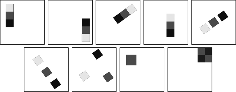
FIGURE 11.13
Query of a three-color object (top-left) in the synthetic database.

11.4.5.1 Retrieval Performance on Synthetic Images

Recall that the images in the synthetic database contain colored regions in geometric and arbitrary shapes within which uniform samples from the entire color space are represented. In this way, the color matching accuracy can be visually evaluated and the first two penalty terms P_φ and P_G can be individually tested. Furthermore, the same or matching colors form different color compositions by varying their region’s shape, size, and/or inter-region proximities. This allows for testing both individual and mutual penalty terms P_G and P_SCD. Finally, the penalty-trio’s cumulative accuracy and robustness against variations of resolution, translation, and rotation can also be tested and compared against the correlogram.

Figure 11.13 presents a snapshot of the query of an image with three-color squares on a white background. The color descriptor is used with proximity histogram as the SCD descriptor and the retrieval results are ranked from left to right and top to bottom and the similarity distances are given on the bottom of the images. Among the first six retrievals, the same amount of identical colors are used and hence P_φ = P_G = 0, which allows for testing the accuracy of P_SCD alone. The first three retrievals have insignificant similarity distances, which demonstrates the robustness of P_SCD against the variations of rotation and translation. The fourth, fifth, and sixth ranks present cases where spatial proximity between the three colors starts to differentiate, and hence SCD descriptor reflects the proximity differences successfully. For the seventh (P_φ ≠ 0) and the eight (P_G ≠ 0) ranks, P_∑ starts to build up significantly, since the color composition changes drastically due to emerging and missing color components.

Images

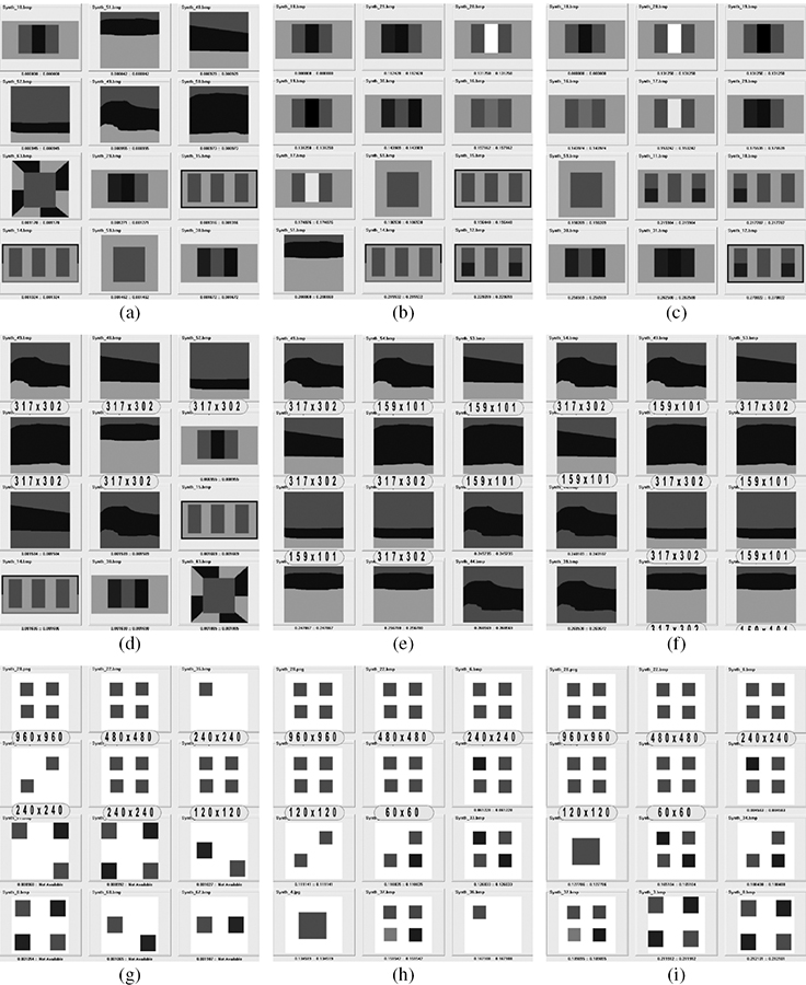
FIGURE 11.14
Three queries in the synthetic database processed using (a,d,g) correlogram, (b,e,h) SCD with proximity histogram, and (c,f,i) SCD with proximity grid. Some dimensions are tagged in boxes below pictures. Top-left is the query image.

Figure 11.14 shows three queries in the synthetic database with different color compositions and resolutions. In the case of Figures 11.14a to 11.14c, both proximity histogram and proximity grid successfully retrieve images with similar color compositions, whereas the correlogram cannot do it due to its invariance to weight (area) and limited range. The area invariance effect can be easily seen in the second and particularly the third ranks, where entirely different red and green weights occur. The same comments can be made in the case of Figures 11.14d to 11.14f for the fifth and all ranks above the seventh. Moreover in this case, it is obvious that the correlogram cannot retrieve the image with identical color composition among the first eleven ranks due to its resolution (pixel-based) sensitivity. Note further that the SCD with both proximity histogram and grid first retrieves the color compositions, where all colors are perfectly matching (P_φ = 0) with the weights in a close vicinity (P_G ≠ 0), and then balances between mismatching colors and weight differences of the matching ones. The case of Figures 11.14g to 11.14i is particularly shown here to emphasize the effect of image resolution over the correlogram and the SCD. The query of the largest image among the others with dimensions in five different resolutions logarithmically scaled from 60 to 960, but the same color composition (four red squares over white background), resulted in accurate ranking for the SCD. On the other hand, the correlogram retrieves accurately only one while the other two are shifted to lower ranks and the one (with 60 × 60 dimension) is missed within the first twelve ranks.

TABLE 11_2
Similarity distances and ranks of A and B in Figure 11.12 when C is queried in Corel 1K database.

Approach	P_∑		Rank
A	B	A	B
with DC fusing	0.176	0.156	3	1
without DC fusing	0.585	0.205	258	1

11.4.5.2 Retrieval Performance on Natural Images

In this section, three sample databases (Corel 1K, Corel 10K, and Corel 20K) are indexed using each FeX module and each individual (sub)feature is used for retrieval. As presented in Table 11.2, the first retrieval experiment is performed to demonstrate the effect of DC fusing over the retrieval accuracy. Similar results of several retrieval experiments suggest that DC fusing becomes the key factor for the success of the SCD. Therefore, DC fusing is applied for the rest of the experiments presented in this section.

TABLE 11.3
ANMRR scores of the SCD and the competing descriptors for databases Corel 1K (34 queries), Corel 10K (176 queries), and Corel 20K (22 queries).

Images

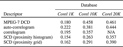
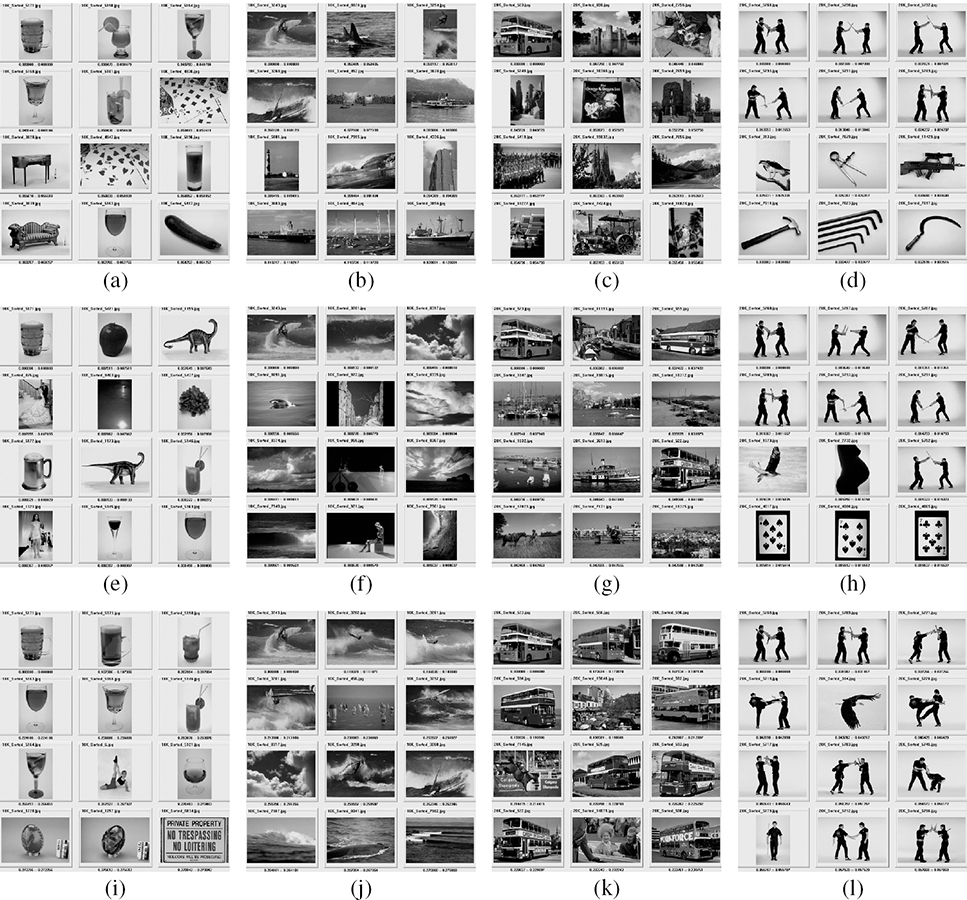
FIGURE 11.15 (See color insert.)
Four typical queries using three descriptors in Corel 10K database: (a–d) dominant color, (e–h) correlogram, and (i–l) proposed method. Top-left is the query image.

Table 11.3 presents ANMRR results and the query dataset size of each of the three Corel databases. The query dataset is prepared a priori by regarding a certain degree of color content coherency. This means that the content similarity can mostly be perceived by color similarity. However, unlike previously presented synthetic images, a unique one-to-one correspondence between content and color similarities can never be guaranteed in natural images due to the presence of other visual cues, such as texture and shape. Nevertheless, according to the presented ANMRR scores, SCD with either mode achieves superior retrieval performance than the competing methods (correlogram, auto-correlogram, and MPEG-7 DCD combined with the quadratic distance computation) for all Corel databases. Moreover, it was observed that in the majority of the queries (between 58 and 78%), the SCD outperforms the (auto-)correlogram, whereas the figure is even higher (76–92%) with the MPEG-7 DCD. Finally, for shorter descriptor size with proximity histograms, a norm was used since comparative retrieval results promise no significant gain of using L₁ (for example, ANMRR score of SCD with proximity histogram using L₁ is 0.254 for Corel 10K).

Images

FIGURE 11.16 (See color insert.)
Four typical queries using three descriptors in Corel 20K database: (a–d) dominant color, (e–h) auto-correlogram, and (i–l) proposed method. Top-left is the query image.

For visual evaluation, four retrieval results are presented for both Corel 10K and Corel 20K databases using all three descriptors. For the queries as shown in Figure 11.15, the proximity grid in SCD was used against the correlogram and MPEG-7 DCD. In the first, second, and fourth queries, one can easily notice the erroneous retrievals of the correlogram due to its color area insensitivity (for instance, compare the amount of red, white, and black colors between the query and the fifth ranked image in the first query). As already discussed, in such large databases the co-occurrence probabilities can (accidentally) match images with significantly different color proportions. Particularly in the first and fourth queries, erroneous retrievals of MPEG-7 DCD occur due to the lack of SCD description, which also makes accidental matches between dissimilar images with close color proportions (for instance, in the first query, the amount of white, red, and black colors is quite close between the query and sixth, seventh, and eight ranks; however, their SCDs are not).

For the queries shown in Figure 11.16, the proximity histogram in SCD was used against the auto-correlogram and the MPEG-7 DCD. Similar conclusions as before can be drawn for the retrieval results. Furthermore, it should be noted that the amount of erroneous retrievals is increased particularly in the second and third queries, since the database size is doubled and hence accidental matches occur more often than before. However, in both databases, the (auto-)correlogram may occasionally perform better than SCD; the case of the queries shown in Figure 11.17, where significant (color) textures are present in all query images. This is indeed in accordance with the earlier remark stating that the correlogram is a colored texture descriptor and hence it can outperform any color descriptor whenever a textural structure is dominant.

Images

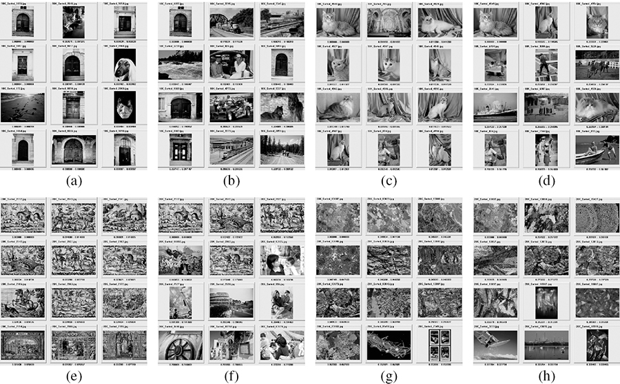
FIGURE 11.17 (See color insert.)
Two queries in (a,b,e,f)Corel 10K and (c,d,g,h)Corel 20K databases where (auto-)correlogram performs better than SCD: (a,e) correlogram, (b,f) proposed method, (c,g) auto-correlogram, and (d,h) proposed method. Top-left is the query image.

11.5 Conclusion

This chapter presented two perceptual and spatial color descriptors. The first one, the perceptual correlogram is primarily designed to overcome the drawbacks of the color correlogram and brings a solution to its infeasibility problems. Utilization of dynamic color quantization instead of a static color space quantization not only achieves a more perceptual description of the color content, but also significantly decreases the number of colors. By doing so, the size of the correlogram table is reduced to feasible limits and since the memory limitations are also suppressed, implementation with higher-range values has become possible. However, it should be still noted that such a pixel-based proximity measure is highly resolution dependent, and if large image resolutions are considered, increasing the range value would become a restrictive factor in terms of memory and speed. Since a dynamic color quantization is applied, the obtained DCs do not have fixed centroids as in static quantization. Therefore, during the retrieval phase, such colors were compared using a one-to-one color matching scheme, which is preferred due to its accurate and fast computation. Yet much complex color matching methods are also possible, such as one-to-many matching, that involves comparison and/or combination of many global and spatial features. Apart from efficient and perceptual description of the color content, using spatial differences only, particularly in terms of probabilities, leaves a color descriptor incomplete. Retrieval experiments on the synthetic databases also demonstrate that global properties are indispensable in judging the color content similarity. These experiments further reveal that the penalty-trio model effectively combines spatial and global features into a similarity distance metric. Although the main aim of this descriptor was to solve the infeasibility problems of the traditional correlogram, the induced perceptuality and addition of global properties further increased the discrimination power. Experimental results, including the ANMRR scores, also demonstrate such superiority. However, it should be noted that color alone does not fully describe the entire image content and it can be associated with it only in a certain extent.

The spatial color descriptor (SCD) presented next in this chapter characterizes the perceptual properties of the color composition in a visual scenery in order to maximize the description power. In other words, the so-called outliers, which are the imperceivable color elements, are discarded for description efficiency using a top-down approach while extracting global and spatial color properties. In this way, severe problems and limitations of traditional pixel-based methods are effectively avoided and in spatial domain only the perceived (visible) color components can be truly extracted using QT decomposition. In order to reveal the true SCD properties, the proximity histogram and the proximity grid, representing the inter-proximity statistics in scalar and directional modes, are presented. During the retrieval phase, one-to-many DC matching is performed in order to apply the penalty-trio model over matching (and possibly fused) DC sets. This greatly reduces the faulty mismatches and erroneous similarity distance computations. The penalty-trio model computes the normalized differences in both spatial and global color properties and combines all so as to yield a complete comparison between two color compositions. Experimental results approve the superiority of the SCD over the competing methods in terms of discrimination power and retrieval performance especially over large databases. The SCD has a major advantage of being applicable to any database size and image resolution. Thus, it does not suffer from the infeasibility problems and severe limitations of the correlogram. Finally, it achieves a significant performance gain in terms of ANMRR scores. However, this gain remained below higher performance expectations, particularly when compared with the correlogram due to two reasons. First and foremost, the correlogram has the advantage of describing texture in color images thanks to its pixel-level analysis via co-occurrence probabilities. Yet the major reason is that the color similarity alone does not really imply the content-similarity. This significantly degrades the retrieval performance of SCD in several experiments. For instance, when an image with gray horse on a green field and a blue sky is queried, all retrievals with a gray elephant and similar background are counted as irrelevant (since they do not belong to horse class), although the color distribution is quite similar. Many other irrelevant retrievals with similar color properties can be seen in the figures presented above. In summary, color properties correlate with the true content only in a certain extent and cannot be used as the single cue to characterize the entire content [47].

Acknowledgment

This chapter is adapted from Reference [48] with the permission from Elsevier.

References

[1] E. van den Broek, P. Kisters, and L. Vuurpijl, “The utilization of human color categorization for content-based image retrieval,” Proceedings of SPIE, vol. 5292, pp. 351–362, January 2004.

[2] A. Mojsilovic, J. Kovacevic, J. Hu, R. Safranek, and K. Ganapathy, “Matching and retrieval based on the vocabulary and grammar of color patterns,” IEEE Transactions on Image Processing, vol. 9, no. 1, pp. 38–54, January 2000.

[3] A. Mojsilovic, J. Hu, and E. Soljanin, “Extraction of perceptually important colors and similarity measurement for image matching, retrieval, and analysis,” IEEE Transactions on Image Processing, vol. 11, no. 11, pp. 1238–1248, November 2002.

[4] K.H. Brandenburg, “MP3 and AAC explained,” in Proceedings of the AES 17th International Conference on High-Quality Audio Coding, Florence, Italy, September 1999.

[5] J. Huang, S. Kumar, M. Mitra, W. Zhu, and R. Zabih, “Image indexing using color correlo-grams,” in Proceedings of the IEEE Conference on Computer Vision and Pattern Recognition San Juan, Puerto Rico, June 1997, pp. 762–768.

[6] I. Kunttu, L. Lepisto, J. Rauhamaa, and A. Visa, “Image correlogram in image database indexing and retrieval,” in Proceedings of the 4th European Workshop on Image Analysis for Multimedia Interactive Services, London, UK, April 2003, pp. 88–91.

[7] W. Ma and H. Zhang, “Benchmarking of image features for content-based retrieval,” in Proceedings of the Thirty-Second Asilomar Conference on Signals, Systems, and Computers, Pacific Grove, CA, USA, November 1998, vol. 1, pp. 253–256.

[8] G. Pass, R. Zabih, and J. Miller, “Comparing images using color coherence vectors,” in Proceedings of the Fourth ACM International Conference on Multimedia, Boston, MA, USA, November 1996, pp. 65–73.

[9] C. Tomasi and R. Manduchi, “Bilateral filtering for gray and color images,” in Proceedings of the International Conference on Computer Vision, Bombay, India, January 1998, pp. 839–846.

[10] M. Wertheimer, “Laws of organization in perceptual forms,” in A Source Book of Gestalt Psychology, London, UK: Routledge & Kegan Paul, 1938, pp. 71–88.

[11] “Muvis,” Available online, http://muvis.cs.tut.fi.

[12] J. Hafner, H. Sawhney, W. Equitz, M. Flickner, and W. Niblack, “Efficient color histogram indexing for quadratic form distance functions,” IEEE Transactions on Pattern Analysis and Machine Intelligence, vol. 17, no. 7, pp. 729–736, July 1995.

[13] I. Cox, M. Miller, S. Omohundro, and P. Yianilos, “Pichunter: Bayesian relevance feedback for image retrieval,” in Proceedings of the IEEE International Conference on Pattern Recognition, Vienna, Austria, August 1996, vol. 3, pp. 361–369.

[14] A. Pentland, R. Picard, and S. Sclaroff, “Photobook: Tools for content-based manipulation of image databases,” Proceedings of SPIE, vol. 2185, pp. 34–47, April 1994.

[15] J. Smith and S. Chang, “Visualseek: A fully automated content-based image query system,” in Proceedings of the Fourth ACM International Conference on Multimedia, Boston, MA, USA, November 1996, pp. 87–98.

[16] “Virage,” Available online, http://www.virage.com.

[17] S. Sclaroff, L. Taycher, and M.L. Cascia, “Imagerover: A content-based image browser for the World Wide Web,” in Proceedings of the IEEE Workshop on Content-Based Access of Image and Video Libraries, San Juan, Puerto Rico, June 1997, pp. 2–9.

[18] S. Chang, W. Chen, J. Meng, H. Sundaram, and D. Zhong, “Videoq: An automated content based video search system using visual cues,” in Proceedings of the Fifth ACM International Conference on Multimedia, Seattle, WA, USA, November 1997, pp. 313–324.

[19] K. van de Sande, T. Gevers, and C. Snoek, “Evaluation of color descriptors for object and scene recognition,” IEEE Transactions on Pattern Analysis and Machine Intelligence, vol. 32, no. 9, pp. 1582–1596, September 2010.

[20] T. Kato, T. Kurita, and H. Shimogaki, “Intelligent visual interaction with image database systems – Toward the multimedia personal interface,” Journal of Information Processing, vol. 14, no. 2, pp. 134–143, April 1991.

[21] M. Swain and D. Ballard, “Color indexing,” International Journal of Computer Vision, vol. 7, no. 1, pp. 11–32, November 1991.

[22] Y. Gong, C.H. Chuan, and G. Xiaoyi, “Image indexing and retrieval based on color histograms,” Multimedia Tools and Applications, vol. 2, no. 2, pp. 133–156, March 1996.

[23] V. Ogle and M. Stonebraker, “Chabot: Retrieval from a relational database of images,” Computer, vol. 28, no. 9, pp. 40–48, September 1995.

[24] J. Smith and S. Chang, “Single color extraction and image query,” in Proceedings of the IEEE International Conference on Image Processing, Washington, DC, USA, October 1995, vol. 3, pp. 528–531.

[25] A. Utenpattanant and O. Chitsobhuk, “Image retrieval using Haar color descriptor incorporating with pruning techniques,” in Proceedings of the 9th International Conference on Advanced Communication Technology, Phoenix Park, Korea, February 2007, vol. 2, pp. 1123–1126.

[26] S. Wang, L.T. Chia, and R. Deepu, “Image retrieval using dominant color descriptor,” in Proceedings of the International Conference on Imaging Science, Systems and Technology, Las Vegas, NV, USA, June 2003, vol. 1, pp. 107–110.

[27] K.M. Wong, L.M. Po, and K.W. Cheung, “A compact and efficient color descriptor for image retrieval,” in Proceedings of the IEEE International Conference on Multimedia and Expo, Beijing, China, July 2007, pp. 611–614.

[28] B. Manjunath, J.R. Ohm, V. Vasudevan, and A. Yamada, “Color and texture descriptors,” IEEE Transactions on Circuits and Systems for Video Technology, vol. 11, no. 6, pp. 703–715, June 2001.

[29] L. Tran and R. Lenz, “Compact colour descriptors for colour-based image retrieval,” Signal Processing, vol. 85, no. 2, pp. 233–246, February 2005.

[30] M. Stricker and M. Orengo, “Similarity of color images,” Proceedings of SPIE, vol. 2420, pp. 381–392, February 1995.

[31] L.M. Po and K.M. Wong, “A new palette histogram similarity measure for MPEG-7 dominant color descriptor,” in Proceedings of the International Conference on Image Processing, Singapore, October 2004, vol. 3, pp. 1533–1536.

[32] G. Babu, B. Mehtre, and M. Kankanhalli, “Color indexing for efficient image retrieval,” Multimedia Tools and Applications, vol. 1, no. 4, pp. 327–348, November 1995.

[33] Y. Deng, C. Kenney, M. Moore, and B. Manjunath, “Peer group filtering and perceptual color image quantization,” in Proceedings of the 1999 IEEE International Symposium on Circuits and Systems, Orlando, FL, USA, June 1999, vol. 4, pp. 21–24.

[34] J. Fauqueur and N. Boujemaa, “Region-based image retrieval: Fast coarse segmentation and fine color description,” Journal of Visual Languages & Computing, vol. 15, no. 1, pp. 69–95, February 2004.

[35] J. MacQueen, “Some methods for classification and analysis of multivariate observations,” in Proceedings of the Fifth Berkeley Symposium on Mathematical Statistics and Probability, Berkeley, CA, USA, 1967, vol. 1, pp. 281–297.

[36] M. Sudhamani and C. Venugopal, “Grouping and indexing color features for efficient image retrieval,” International Journal of Applied Mathematics and Computer Sciences, vol. 4, no. 3, pp. 150–155, May 2007.

[37] I. Valova and B. Rachev, “Retrieval by color features in image databases,” in Proceedings of the European Conference on Advances in Databases and Information Systems, Budapest, Hungary, September 2004.

[38] B. Ooi, K.L. Tan, T. Chua, and W. Hsu, “Fast image retrieval using color-spatial information,” VLDB Journal, vol. 7, no. 2, pp. 115–128, May 1998.

[39] A. Nagasaka and Y. Tanaka, “Automatic video indexing and full-video search for object appearances,” in Proceedings of the Second Working Conference on Visual Database Systems, Budapest, Hungary, October 1991, pp. 113–127.

[40] H. Lee, H. Lee, and Y. Ha, “Spatial color descriptor for image retrieval and video segmentation,” IEEE Transactions on Multimedia, vol. 5, no. 3, pp. 358–367, September 2003.

[41] J. Luo and D. Crandall, “Color object detection using spatial-color joint probability functions,” IEEE Transactions on Image Processing, vol. 15, no. 6, pp. 1443–1453, June 2006.

[42] T. Ojala, M. Rautiainen, E. Matinmikko, and M. Aittola, “Semantic image retrieval with HSV correlograms,” in Proceedings of the 12th Scandinavian Conference on Image Analysis, Bergen, Norway, June 2001, pp. 621–627.

[43] Y. Chun, N. Kim, and I. Jang, “Content-based image retrieval using multiresolution color and texture features,” IEEE Transactions on Multimedia, vol. 10, no. 6, pp. 1073–1084, October 2008.

[44] J. Li, W. Wu, T. Wang, and Y. Zhang, “One step beyond histograms: Image representation using markov stationary features,” in Proceedings of the IEEE International Conference on Computer Vision and Pattern Recognition, Anchorage, AK, USA, June 2008, pp. 1–8.

[45] S.J. Lee, Y.H. Lee, H. Ahn, and S.B. Rhee, “Color image descriptor using wavelet correlogram,” in Proceedings of the the 23rd International Technology Conference on Circuits/Systems, Computers and Communications, Shimonoseki, Japan, July 2008, pp. 1613–1616.

[46] H. Moghaddam and M. Saadatmand-Tarzjan, “Gabor wavelet correlogram algorithm for image indexing and retrieval,” in Proceedings of the IEEE International Conference on Pattern Recognition, Hong Kong, August 2006, vol. 2, pp. 925–928.

[47] B. Rogowitz, T. Frese, J. Smith, C. Bouman, and E. Kalin, “Perceptual image similarity experiments,” Proceedings of SPIE, vol. 3299, pp. 576–590, January 1998.

[48] S. Kiranyaz, M. Birinci, and M. Gabbouj, “Perceptual color descriptor based on spatial distribution: A topdown approach,” Image and Vision Computing, vol. 28, no. 8, pp. 1309–1326, August 2010.

..................Content has been hidden....................

You can't read the all page of ebook, please click here login for view all page.

Table of Contents for 11 Perceptual Color Descriptors

Create new playlist

Sign In

Sign Up

Table of Contents for
11 Perceptual Color Descriptors