7
Perceptual Thumbnail Generation
Wei Feng, Liang Wan, Zhouchen Lin, Tien-Tsin Wong and Zhi-Qiang Liu
7.2 Traditional Thumbnail Generation
7.2.1 Signal-Level Thumbnail Generation
7.2.2 ROI-Based Thumbnail Generation
7.3 Perceptual Thumbnail Generation
7.3.1 Quality-Indicative Visual Cues
7.3.1.1 Low-Level Image Features
7.3.1.2 High-Level Semantic Features
7.3.3 State-of-the-Art Methods
7.4 Highlighting Blur in Thumbnails
7.4.1.1 Gradient-Based Blur Estimation
7.4.1.2 Scale-Space-Based Blur Estimation
7.5 Highlighting Noise in Thumbnails
7.5.1.1 Region-Based Noise Estimation
7.5.1.2 Multirate Noise Estimation
7.1 Introduction
As shrunk versions of pictures, thumbnails are commonly used in image preview, organization, and retrieval [1], [2], [3], [4]. In the age of digital media, a thumbnail plays a similar role for an image as an abstract does for an article. Just consider today’s digital cameras; it is hard to find one with less than six Megapixels. Viewers expect to observe both the global composition and important perceptual features of the original full-size picture by inspecting its thumbnail, which should thus provide a faithful impression about the image content and quality.
In practice, thumbnails mainly serve in the following two aspects. First, they provide viewers a convenient way to preview high-resolution pictures on a small display screen. For instance, many portable devices, such as digital cameras and cell phones, provide prompt image preview function by small-size LCD displays [5]. Second, thumbnails enable the user to quickly browse a large number of images without being distracted by unimportant details. For example, almost all visual search engines, such as Google Images and Bing Images, use thumbnails to organize their returned search results. As the proliferation of digital images has been increasing in recent years, generating perceptually faithful thumbnails becomes very important.
From the historical viewpoint, the concept of thumbnail is gradually changed due to the developing practical requirements in real-world applications. At the very beginning, for a given full-size picture, a thumbnail was generated simply by filtering and subsampling [6], [7]. Then, to emphasize some important portions in original pictures, region of interest (ROI)-based thumbnails were proposed based on visual attention models [1], [8]. Compared to conventional downsampled thumbnails that equally treat all image parts and features in the original size, ROI-based thumbnails highlight visually important regions only, thus helping viewers to focus on essential parts, but inevitably losing the perceptual faith of global composition in original pictures. In recent years, moreover, people start to realize the necessity and importance of perceptual thumbnails [5], [9]. Specifically, perceptual thumbnails highlight the quality-related and perceptually important features in original pictures, with the global structural composition preserved. From perceptual thumbnails, viewers can easily assess the image quality without checking the original full-size versions, thus facilitating faithful image preview on small displays and fast browsing of a large number of pictures. In contrast, without perceptual thumbnails, evaluating the quality of images taken by digital cameras requires that the user has to repeatedly zoom in, zoom out at different scales, and shift across different parts of the pictures at higher resolutions, which is usually very time consuming, inconvenient, and ineffective. Moreover, the operation of zooming in may also make viewers lose the perception of the global composition of pictures.
Clearly, both conventional downsampled thumbnails and ROI-based thumbnails are not qualified to serve as perceptual thumbnails. As shown in Figure 7.1, some apparent perceptual features in the original pictures, for instance, blur and noise, may easily be lost in the downsampled thumbnails, no matter what interpolation algorithm is used. As mentioned above, the conventional downsampling process may significantly reduce the resolution of perceptual features in downsampled thumbnails. To discover a phenomenon in an image, the resolution of the phenomenon must be larger than some threshold that represents the perceiving capability of viewers. When the reduced resolution of naively downsampled perceptual features becomes less than viewers’ perceiving thresholds, these features cannot be noticed. Therefore, in perceptual thumbnails, some important quality-related features should be highlighted and the resolution of perceptual features should not be affected by the downsampling process. Besides, ROI-based thumbnails cannot be used as perceptual thumbnails since this approach destroys the global composition of the original pictures. To this end, successful perceptual thumbnail generation should meet the four requirements discussed below.
Low cost: As thumbnails are widely used in prompt preview of high-resolution pictures and fast browsing of a large number of images, they must be generated in an economic way in terms of their computation and storage. Hence, fast and simple algorithms for highlighting perceptual features are desirable.
Unsupervision: Since one may want to quickly produce a large number of thumbnails in a browsing task, they should be generated automatically. Both preliminary training and on-the-fly parameter tuning should be avoided.
Highlighting multiple perceptual features: To faithfully reflect the content and quality of original full-size pictures in thumbnails, multiple quality-related features, such as blur and noise, should be highlighted according to their respective strengths.
Preserving the original composition: It is important for perceptual thumbnails to provide viewers with a clear impression about the global structure (composition) of original pictures. For instance, the user may want to quickly decide whether or not to take a second shot of the same scene by checking the thumbnails on small display screens in their cameras.
This chapter focuses on introducing the recent development of perceptual thumbnail generation techniques that satisfy the above four requirements. Within a unified framework, particular attention is paid to preserving and highlighting two types of quality-related perceptual features, that is, blur and noise.
Section 7.2 briefly introduces the techniques for traditional thumbnail generation and specifically discusses signal-level downsampled thumbnail generation and ROI-based thumbnail generation methods. Signal-level thumbnail generation concerns the development of different filtering or interpolation techniques in order to reduce aliasing artifacts in thumbnails. In contrast, ROI-based thumbnail generation aims at preserving salient image regions and essential structures during image resizing.
The next three sections focus on the technical details of perceptual thumbnails. Namely, Section 7.3 first described the commonly noticed visual cues/features that indicate image quality and need to be preserved in perceptual thumbnails. Then, it introduces a general framework for perceptual thumbnail generation, focused on blur and noise as two commonly encountered types of low-level perceptual features. This framework can be extended to include other types of perceptual features, such as bloom and overexposure. At last, this section briefly presents several state-of-the-art perceptual thumbnail generation methods that are based on the proposed general working flow. Sections 7.4 and 7.5 elaborate how to highlight spatially variant blur and homogeneous noise in thumbnails, respectively. Although blur and noise estimation has been studied for decades in image processing and computer vision, most previous deblurring and denoising methods tried to get an accurate estimate of blur and noise strength for the goal of recovering blur-free and noise-free images. Perceptual thumbnail generation, on the contrary, aims to highlight blur and noise at a noticeable scale in thumbnails. This raises the requirements of appropriate but inexact algorithms for blur and noise estimation, as well as alias-free blur and noise visualization. Therefore, these two sections also discuss how to quickly estimate blur and noise from the original images, and effectively visualize them in the downsampled thumbnails.
Section 7.6 presents a number of experimental results that comprehensively compare the performance of different techniques in perceptual thumbnail generation. Current perceptual thumbnail generation only handles blur and noise, the two low-level visual cues. Finally, this chapter concludes with Section 7.7, which summarizes the state-of-the-arts of perceptual thumbnail generation and discusses some possible ways to highlight other types of perceptual cues, including red-eye effect and bloom, in thumbnails.
7.2 Traditional Thumbnail Generation
Traditional thumbnail generation techniques can be classified as signal-level thumbnail generation and ROI-based thumbnail generation. Signal-level thumbnail generation techniques [7], [10], [11], [12], [13] create the thumbnail from a high-resolution original image by prefiltering and subsampling. The generated thumbnail preserves the original composition. ROI-based thumbnail generation techniques [2], [3], [14], [15], [16], on the other hand, aim at detecting and retaining important regions in the resulting thumbnail.
7.2.1 Signal-Level Thumbnail Generation
Signal-level thumbnail generation relies on image resampling techniques, which usually employ both filtering and subsampling [17]. Due to different filtering schemes employed, the quality of the resulting thumbnails may differ greatly. Among the existing image resampling techniques, the simplest method is decimation, that is, keeping some pixels of the original image and throwing others away. Without prefiltering the original image, decimation typically leads to significant aliasing artifacts.
To reduce such aliasing artifacts, lowpass filters can be used before decimation. For example, box filter computes an average of pixel values within the pixel neighborhood. Bilinear filter performs linear filtering first in one direction, and again in the other direction. The bicubic filter [10] is often chosen over the bilinear filter since the resampled image is smoother and has fewer aliasing artifacts. Other than second-order polynomials defined in bilinear filter and third-order polynomials defined in bicubic filter, high-order piecewise polynomials [12] can also be used, although the improvement is marginal. More sophisticated B-spline approximation is reported in the literature for image resampling [7], [11]. There exist other suitable linear methods, including Lanczos [6] and Mitchell [18] filters. The aforementioned filters are space-invariant (isotropic) in nature. In the context of texture mapping, perspective mapping leads to space-variant (anisotropic) footprint. For this application, elliptic Gaussian-like filters have been employed [19], [20], [21].
Another trend of image resampling is to perform edge-adaptive interpolation in order to generate sharp edges in the resampled image. In Reference [22], the authors developed an edge-directed image interpolation (NEDI) algorithm. They estimated local covariance from a low-resolution image and used the low-resolution covariance to adapt the image interpolation at a higher resolution. Reference [23] developed a method to optimally determine the local quadratic signal class for the image. Reference [24] proposed an edge-guided nonlinear interpolation algorithm, which estimates two observation sets in two orthogonal directions, and then fuses the two observation sets by the linear minimum mean square-error estimation technique. Another work [25] relied on a statistical edge dependency relating edge features of two different resolutions, and solved a constrained optimization. It should be noted that edge-adaptive resampling techniques are specially designed for image upsampling, and they are usually not suitable for image downsampling.
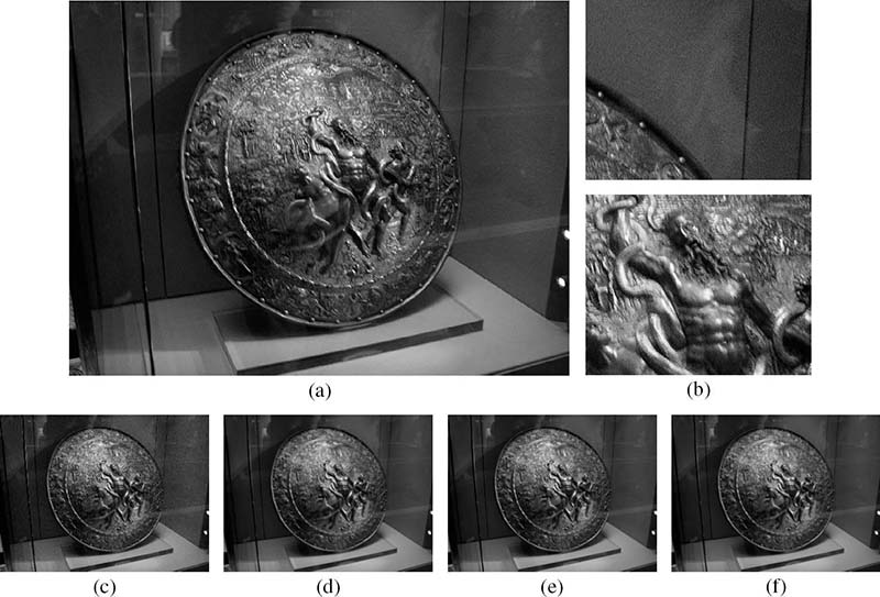
FIGURE 7.1 (See color insert.)
Signal-level thumbnail generation: (a) original image, (b) two magnified regions cropped from the original image, and (c–f) thumbnails. Thumbnails are downsampled using (c) decimation, (d) bilinear, (e) bicubic, and (f) Lanczos filtering.
Figure 7.1 illustrates several commonly used image resampling methods. The original image has a resolution of 2048 × 1536 pixels, and is downsampled to a resolution of 320 × 240 pixels. As shown in Figure 7.1c, decimation results in severe aliasing artifacts. Bilinear filtering, shown in Figure 7.1d, removes artifacts. Bicubic filtering, shown in Figure 7.1e, produces a smoother thumbnail by further reducing the aliasing artifacts. The thumbnail generated using Lanczos filtering, shown in Figure 7.1f, has even fewer artifacts; however, this method is much slower than others. Obviously, signal-level thumbnail generation techniques can prevent aliasing artifacts and preserve the original image composition. However, they are not designed to preserve perceptual image quality during image resampling. In fact, they probably lose such features that are useful to the user to identify the image quality. Visual inspection of the magnified regions in Figure 7.1b reveals that the original high-resolution image suffers from noticeable blur and noise. However, the three thumbnails in Figures 7.1d to 7.1f all appear rather clean and clear. A qualitative analysis of the loss in the blur and noise will be presented in Section 7.3.
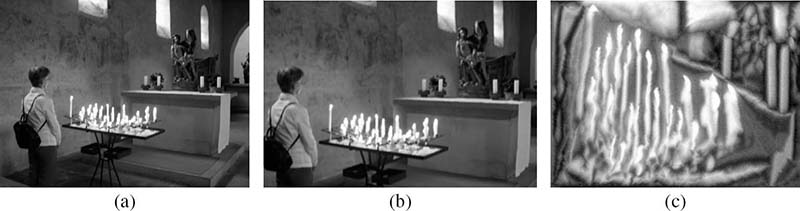
FIGURE 7.2 (See color insert.)
ROI-based thumbnail generation: (a) high-resolution image, (b) automatic cropping, and (c) seam carving.
7.2.2 ROI-Based Thumbnail Generation
Unlike signal-level thumbnail generation, which preserves the original image composition, ROI-based thumbnail generation (Figure 7.2) just displays important image regions in the small-scale thumbnail. In Reference [1], the downsampling distortion was reduced by treating the high-resolution original image with edge-preserving smoothing, lossy image compression, or static codebook compression. Reference [8] used an image attention model based on region of interest, attention value, and minimal perceptible size to incorporate user attention in the process of adapting the high-resolution image on small-size screens. For screens with different scale and aspect ratio, different important regions were cropped from the original image for downsampling. Similarly, Reference [14] detected key components of the high-resolution image based on a saliency map, and then cropped images prior to downsampling (Figure 7.2c). Although the cropping-based methods can render important image portions in a more recognizable way, the user will lose the global overview of the original image.
Another research direction relating to thumbnail generation is image retargeting, which considers geometric constraints and image contents in the resizing process. Reference [26] maximized salient image objects by minimizing less important image portions in-between. Since the spatial spaces between image objects may be narrowed, the relative geometric relation between the objects can be altered in the thumbnail. Reference [15] presented a seaming carving approach (Figure 7.2c), which removes or inserts an eight-connected path of pixels on an image from top to bottom, or from left to right in one pass. This method, though quite simple, is rather time consuming and may damage the image structure severely. To address the problems in seaming carving, various retargeting techniques [16], [27], [28], [29] have been proposed. Although the techniques can be quite different, their objectives are similar: preserving the important image content, reducing visual artifacts, and preserving internal image structures. A comprehensive evaluation of state-of-art methods can be found in Reference [30].
Additionally, special concerns have been reported to address the situation when the highresolution image contains texts. For example, Reference [3] created thumbnails for web pages by combining text summaries and image thumbnails. Reference [2] cropped and scaled image and text segments from the original image and generated a more readable layout for a particular display size. Following the aforementioned two works, many subsequent research works can be found, such as References [31], [32], and [33].
The ROI-based thumbnail generation techniques have been proven successful in preserving important image contents in the low-resolution thumbnail. However, none of them account for perceptual quality features in the high-resolution image. As a result, such techniques may remove these desired features during image downsizing.
7.3 Perceptual Thumbnail Generation
This section first describes several common visual/perceptual cues that indicate image quality. Then, it presents a general framework for perceptual thumbnail generation, specifically focusing on highlighting blur and noise in thumbnails. Finally, a brief overview of the state-of-the-art methods in perceptual thumbnail generation is presented.
7.3.1 Quality-Indicative Visual Cues
Given a picture shot with a digital camera, the user often demands to inspect whether or not the picture is well shot by quickly checking the thumbnail image. Such a quality inspection process can certainly benefit from properly highlighting some perceptual features in the thumbnail. However, in order to do so, one first needs to find what features or effects in the original picture should be highlighted in the thumbnail. According to practical photography experiences, there are generally two categories of quality-related perceptual features: low-level image features and high-level semantic features.
7.3.1.1 Low-Level Image Features
There are some features that degrade the quality of an image but have less to do with the image content. Such features include blur, noise, bloom, overexposure, underexposure, and so on. In most cases, these features are quality indicative and should be noticed by the user during the photo-taking process, thus requiring to be preserved and highlighted by the downsampling operation when creating the thumbnails.
Blur: Except for some special cases, a blurry picture is usually inferior to a sharp picture of the same scene. The user often accidently moves his or her hands during photo shooting, thus creating blur, which may also occur when there are moving objects in the scene or when some subjects are out of focus of the camera. Image blur, such as spatially varying blur and homogeneous blur, caused by different reasons may exhibit different spatial properties. In most cases, if the user notices unexpected blur in a picture through the preview screen of a digital camera, the user may choose to take a second shot on the same scene. Hence, blur is a very important quality-indicative effect in images and certainly should be highlighted in perceptual thumbnails. An example of image blur is shown in Figure 7.3a.
Noise: Image noise is the random variation of color or brightness information produced by image sensors during exposure and analog-to-digital conversion. It often looks like color grains and scatters over the entire image. There are two types of image noise: fixed pattern noise and random noise [34]. Fixed pattern noise is generally visible when using long exposure time or when shooting under low-light conditions with high ISO speed. It has the same pattern under similar lighting conditions. Random noise occurs at all exposure times and light levels. It appears as randomly fluctuated intensities and colors, and is different even under the identical lighting condition. Banding noise is a special type of random noise that appears as horizontal or vertical strikes. It is generated by the camera when reading data from image sensors, and is more noticeable at high ISO speed. Generally, any noise degrades the quality of a picture and therefore is also quality indicative. Figure 7.3b demonstrates how image noise appears in a picture.
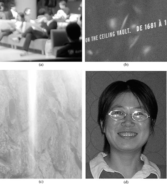
FIGURE 7.3 (See color insert.)
Quality-indicative visual cues: (a) blur, (b) noise, (c) bloom, and (d) red-eye defects.
Bloom: Bloom is the phenomenon that a bright light source appears as a bright halo and leads to color bleeding into nearby objects. This phenomenon occurs when the light source is so strong that the sensor pixels become saturated. For example, in Figure 7.3c, shooting direct sunlight will generate such effect around the boundary of sunlight area. Since the appearance of bloom will significantly destroy the local details of a scene, bloom is also quality indicative.
Overexposure and underexposure: Overexposure and underexposure refer to the effect of losing details in highlight and shadow regions, respectively. This is usually caused by inappropriate setting of camera’s shutter speed and exposure. In highresolution photography, except for some special effects, overexposure and underexposure should be avoided in order to maintain high image quality.
7.3.1.2 High-Level Semantic Features
High-level perceptual features are highly related to the image content [35], as they either reflect some unexpected phenomena of the particular objects or even relate to some aesthetic aspects of the image. Some typical high-level perceptual features are listed below. High-level perceptual features are more difficult to be detected and highlighted in thumbnails than low-level perceptual features.
Defected eyes: When shooting a human subject, the user usually cares whether the eyes were opened at the time of pressing the camera shutter and do not appear as red due to the reflected light from the flash (Figure 7.3d). To automatically detect and correct the red-eye effects in images, various methods have been designed [36], [37].
Simplicity: The most discriminative factor that differentiates professionals from amateur photographers is whether the photo is simple [35]. For a picture, being simple usually means that it is easy to separate the subject from the background. There are various ways for professionals to achieve this goal, including making background out of focus, choosing significant color contrast, and using large lighting contrast between the subject and the background. Recently, simplicity was also used as an important criterion for image quality assessment [35].
Realism: Similar to simplicity, realism is another high-level feature that reflects aesthetic image quality [35]. Professional photographers often carefully choose the lighting conditions and the color distribution, and make use of filters to enhance the color difference. They are also very deliberate in the picture composition of the subject and background. All these are for the purpose of keeping the foreground of pictures as realistic as possible.
In the context of thumbnail generation, some features (for example, simplicity and realism) might remain in the low-resolution thumbnail to some extent, while other features (for example, blur, noise, bloom, overexposure/underexposure, and defected eyes) are less noticeable due to the downsampling process. This chapter focuses on studying how to preserve two typical low-level image features, that is, blur and noise, in thumbnails. As already mentioned, these two phenomena may significantly degrade image quality and commonly exist in digital pictures.
7.3.2 A General Framework
Before presenting the general framework of producing perceptual thumbnails, the loss of blur and noise features by conventional image downsampling is first analyzed. Suppose the original image is represented as vector x. Denote the antialiasing lowpass filter as T and subsampling operation as S. The conventional thumbnail can then be expressed as follows:
where ∘ stands for function composition. When the original image suffers from blur and noise, it can be formulated as
where B and n represent the blur and noise, respectively, and is the ideal image without blur and noise degradation. Substituting Equation 7.2 into Equation 7.1 gives
The following examines the term of the above equation. Except for some extreme blurs, the lowpass filter B, usually representing accidental blur, has a much larger bandwidth than the lowpass filter T. In another words, compared to the influence of filter T, the influence of filter B can be much less noticeable in small-resolution thumbnails. Consequently, the conventional downsampled thumbnails will appear rather sharp than at their original scales.
In the second term S ∘ T (n) of the same equation, the noise n, mostly composed of lots of high-frequency information, is filtered by T. Thus, it will become much less apparent than in the original resolution. For instance, if n is a Gaussian noise of zero mean and moderate variance, T (n) will be close to zero under typical downsampling factors. As a result, the conventional thumbnail y will appear rather clean.
To highlight the blur and noise effects in y with proper strength, the perceptual thumbnail can be formulated as follows:
Intuitively, the conventional thumbnail should be blurred according to the blur strength in the original image, and the noise information should be superimposed at the same time. By this way, the user can easily inspect and discover the blur and noise level in the image by viewing the thumbnail alone.
Using the above extract-and-superimpose strategy, the general framework of perceptual thumbnail generation, which is capable of highlighting blur and noise features, can now be summarized. As illustrated in Figure 7.4, the high-resolution image is first downsampled to get the conventional thumbnail. Then, the blur and noise information present in the original high-resolution image is estimated and extracted. Afterward, the detected amount of blur is properly added into the thumbnail, followed by rendering the estimated noise in order to produce the refined perceptual thumbnail. Note that the presented framework for perceptual thumbnail generation is general enough and can be easily extended to include other types of perceptual features.
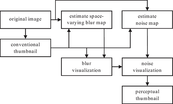
FIGURE 7.4
The framework of perceptual thumbnail generation, which particularly highlights two typical perceptual features, that is, blur and noise. This framework uses the general extract-and-superimpose strategy that can be easily extended to include other types of perceptual features.
7.3.3 State-of-the-Art Methods
Although perceptual thumbnail generation is relatively a new topic, there are several related preliminary works that have been reported in the literature. For instance, the image preview method introduced in Reference [5] divides the problem of perceptual thumbnail generation into structure enhancement and perceptual feature visualization tasks. The first task highlights the salient structure and suppresses the subtle details in the image by non-linearly modulating the image gradient field. The second task estimates the strength of blur and noise in the original image and then superimposes blur and noise with appropriate degrees in the conventional thumbnail. Similarly, Reference [4] studied how to estimate and visualize blur and noise features in the thumbnail. The perceptual thumbnail were generated by directly blurring the conventional thumbnail and adding noise to it. The noise estimation method was further improved to achieve fast performance [9]. Other related efforts in this direction have been exploited in References [38] and [39].
Current perceptual thumbnail generation is highly related to the problems of image deblurring [40], [41], [42] and denoising [43], [44]. These two problems are rather difficult, and the relevant algorithms are usually complicated and time consuming. In contrast, instead of reconstructing the ideal high-resolution image, the goal of perceptual thumbnail generation is to visualize blur and noise in a proper way with reasonable complexity. This relieves the need of recovering actual blur kernels and estimating the noise accurately. Instead, a rough yet fast algorithm for blur and noise estimation is preferable. This is indeed the focus of the existing works related to perceptual thumbnail generation. Although most of these works consider blur and noise in perceptual thumbnails, they adopt quite different algorithms for blur/noise estimation and rendering. The following describes the two representative methods proposed in References [4] and [5].
7.4 Highlighting Blur in Thumbnails
This section suggests how to highlight the reduced blurriness in perceptual thumbnails. Specifically, for the blurred regions in the original high-resolution picture, the perceptual blur highlighting method should magnify the reduced blurriness in their downsampled counterparts, while for the sharp regions at original scales, the goal is to maintain their clearance in thumbnails. Hence, the two major steps in perceptual blur highlighting are blur strength extraction from the original pictures and faithful visualization of extracted blurriness in thumbnails.
7.4.1 Blur Estimation
In the literature, there exist many methods for blur estimation; these methods provide global blur metrics and evaluate the overall blurriness of an image [45], [46], [47]. A suitable global blur metric is helpful to assess images with uniform blurs, such as the motion blur due to shaking cameras. This is, however, insufficient for producing perceptual thumbnails, since the pictures may contain spatially varying blurs. For example, the out-of-focus regions may appear different blur strength at different depth. This raises the demands for local blur estimation. Although there exist studies focused on spatially varying blur determination [48], [49], [50], most of them rely on solving various optimization problems, which is is usually time consuming and inconvenient, and thus these methods are not suitable for efficiently generating perceptual thumbnails. To overcome this drawback, two techniques [5], [9] for roughly determining a local blur strength map from a high-resolution image will now be described.
7.4.1.1 Gradient-Based Blur Estimation
Gradient-based blur estimation [5] relies on an important observation that the variation of a blurry edge region is much more gradual than that of a sharp edge region. Thus, the strength of regional blurriness can be quantitatively measured according to the variance of gradient angles/directions within the corresponding edge region. Specifically, the smaller the regional variance of gradient angles is, the blurrier the edge region would be. To verify this fact, Figure 7.5 shows the simulation test where each of the six high-resolution images were first blurred by Gaussian filters with increased standard deviations and then the variances of gradient directions in all edge regions were measured. As can be seen, as the strength of Gaussian filters increases, the average of directional variances in the gradient field decreases significantly.
Let Ai denote the gradient angle of the i-th edge pixel, which can be obtained as
where Δt (i) and Δs(i) are the first-order differences of pixel i along two spatial dimensions. Then, the gradient-based space-varying blur metric can be defined as follows:
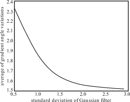
FIGURE 7.5
Inverse relationship of blur strength and regional variance of gradient directions.
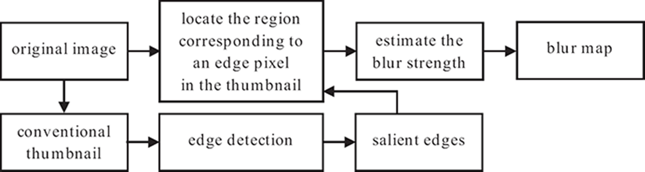
FIGURE 7.6
Gradient-based blur estimation flowchart.
where var(·) is the variance operator and returns the direction variance within the neighborhood of pixel i. Parameters α, β, and τ control the influence of local gradient directional variance to the estimated blur strength. With this equation, the estimated blur strength is increasing with respect to the standard deviation of the Gaussian filter, as will be shown later.
In the context of perceptual thumbnail generation, there is no need to estimate the blur metric for the entire image at the original high resolution. In fact, one needs only to partially measure the blur strength in the low-resolution thumbnail image. Specifically, the blur around edge regions is visually much more noticeable and important to the viewers than in other regions [5], even when the entire image is very blurry. Hence, to speed up the computation, gradient-based blur estimation and highlight can be performed only around the edge regions in the thumbnail image by referring to its original version at the high resolution. As a result, as illustrated in Figure 7.6, gradient-based blur estimation is a three-step process. First, edge detection is performed on the conventional thumbnail to get salient edge pixels. Second, for each edge pixel in the thumbnail, its corresponding region at the original high-resolution picture is found. This small region defines the pixel neighborhood that is used to evaluate the gradient angel variance of current edge pixel. Finally, the blur metric is computed according to Equation 7.6. In this way, a blur strength map for all edge pixels in the thumbnail image can be obtained.
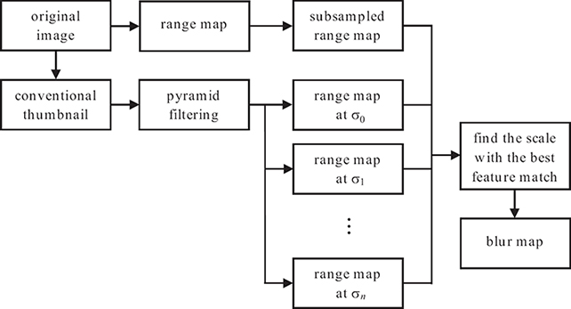
FIGURE 7.7
Scale-space-based blur estimation flowchart.
7.4.1.2 Scale-Space-Based Blur Estimation
Scale-space-based blur estimation [9] generates a space-varying blur map. Its basic idea, in contrast to gradient-based estimation, is first to smooth the conventional thumbnail using various Gaussian kernels with different scales and then to find the best filter scale such that the smoothed region in the filtered thumbnail image is most similar to the corresponding region in the high-resolution image. The algorithmic flow of scale-space-based blur estimation is illustrated in Figure 7.7. In order to generate a space-varying blur map, filter scale matching is performed for the entire thumbnail image. Similar to gradient-based blur estimation, this method does not differentiate between motion blur and out-of-focus blur, and just estimates the pixel-level blur metric. However, unlike gradient-based blur estimation, the scale-space method estimates the blur strength of all pixels in the thumbnail image.
In more detail, the conventional thumbnail y is blurred by a series of Gaussian kernels g with increasing scales [σj}, generating an indexed set of filtered thumbnails fj as follows:
where g(·) represents Gaussian filter. As shown in Figure 7.7, for each blurred thumbnail, a local feature is extracted at each pixel and is compared to the features extracted from the high-resolution image. Here, the local feature of a pixel is defined as the maximum absolute difference between the appearances of the pixel and its surrounding eight neighbors. This generates a series of range maps {rj}, where j is the index of evaluated Gaussian filter scales [9]. Similarly, a range map for the high-resolution image is generated and subsampled to the thumbnail scale by further taking the maximum range value in a high-resolution neighborhood conforming to the subsampling factor. Specifically, denote the subsampled range map to be ro. The blur map index at pixel i can then be computed as
where the parameter γ controls the amount of highlighted blur in thumbnails. Empirically, besides the conventional thumbnail, ten additional scales were used in experiments, starting from σ1 = 0.5 and ending at σ11 = 2.4 with an increment of 0.2111. Note that in the above equation, the blur map returns the index of evaluated Gaussian filters. For illustration purposes, the corresponding blur scale is visualized in Figure 7.7.
7.4.2 Blur Visualization
The second step of perceptual blur highlighting is faithful blur visualization. After performing either gradient-based blur estimation [5] or scale-space-based blur estimation [9], the extracted space-varying blur maps control Gaussian kernels with varying scales, which are finally superimposed into the downsampled thumbnail y pixel by pixel and result in a faithfully blurred thumbnail yb. Note that although the actual image blur in the original resolution may not be exactly conformed to Gaussian kernels, using Gaussian filters in the blur visualization for perceptual thumbnails is empirically a reasonable and effective choice, as the goal is to produce a visually faithful and noticeable blur effect.
Particularly, there are two types of methods to superimpose the space-varying Gaussian blurs in thumbnails. The first method is incremental superimposition. In the case of gradient-based blur estimation [5], the estimated pixel-level blur metric can be used as the standard deviation of a Gaussian filter. Note that the blur is estimated only at edge pixels of the conventional thumbnail. To get a reliable blurring effect, the blur strength at edge pixels is diffused to their neighborhood with self-adjusted filter scales. The blur metric for one pixel near an edge region is approximated as a weighted average of blur strengths of edge pixels nearby. The second method is independent superimposition. For the case of scale-space-based blur estimation [9], the estimated blur value corresponds to a specific Gaussian kernel with a particular scale. Since blur estimation is conducted at the entire thumbnail image, pixel values can be directly selected from the blurred thumbnails as follows:
where mi is the detected index of Gaussian filters for pixel i, and is the smoothed neighborhood of pixel i in the thumbnail image.
Note that both incremental and independent superimposition have respective pros and cons. For instance, independent superimposition tends to produce artifacts in the blurred thumbnails, since there is nothing to protect the spatial coherence of blur strength by independent blur rendering. On the other hand, incremental superimposition has no such problem; however, the exact blur strength rendered into the thumbnail image is not implicitly clear when using incremental superimposition.
7.4.3 Evaluation
A simulation test with uniform blur is conducted to study how the blurriness is preserved across different blur strengthes. Six sharp high-resolution images are chosen as the test dataset. Each high-resolution image is blurred by a series of Gaussian kernels with increasing standard deviations starting from 0.5. The conventional thumbnails that match different blur strengths are prepared as well. Finally, the average blur strength is obtained for each blurred image using gradient-based blur estimation and scale-space-based blur estimation.
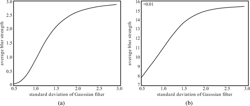
FIGURE 7.8
Relationship between detected blur strength and the ground truth Gaussian filter scales: (a) gradient-based blur estimation and (b) scale-space-based blur estimation.
Figure 7.8 shows the results of the average of the estimated blur standard deviations for the considered dataset. For gradient-based blur estimation, the estimated blur standard deviation is the computed blur metric. For scale-space-based blur estimation, the standard deviation of matched filter is retrieved according to the estimated index of tested Gaussian kernels. In both cases, the estimated standard deviation values increase as the blur gets more severe. In addition, they increase rapidly for small blur scales and become saturated for large blur scales.
7.5 Highlighting Noise in Thumbnails
Highlighting image noise in the thumbnail also involves two major steps, that is, estimating the noise in a high-resolution image and visualizing the noise in the image thumbnail.
7.5.1 Noise Estimation
Traditional image denoising [43], [44], [51] aims at reconstructing a noise-free image from its input noisy version. It is critical to have an accurate estimate of noise, otherwise the recovered image is still degraded. In perceptual thumbnail generation, the goal is to visualize noise and the exact precise form of the noise is not necessary for displaying noise in thumbnails. This relieves the requirement for noise estimation in two aspects. First, some prior knowledge about noise distribution can be exploited. Second, fast and inexact noise estimation methods [5], [9] can be used.
7.5.1.1 Region-Based Noise Estimation
Image noise, as discussed in Section 7.3, is generated by image sensors during image acquisition. It is distributed over the entire image irrespective of the image content. How-ever, image noise is more visually apparent to the viewer in intensity-uniform regions than texture-intensive regions. It is because image noise is a high-frequency signal. Texture regions also have lots of high-frequency details; therefore, differentiating image noise from high-frequency texture details is usually difficult. Uniform regions, on the contrary, contain much less details, and hence the high-frequency information in uniform regions are mainly from image noise. Taking this prior knowledge, a region-based noise estimation was developed in Reference [5]. Its basic idea is to detect noise in a small uniform region of the high-resolution image, and then to synthesize a noise map in the thumbnail resolution based on the estimated noise region. Figure 7.9 illustrates the procedure.

FIGURE 7.9
Region-based noise estimation flowchart.
Region-based noise estimation starts with the conventional thumbnail y and divides it into non-overlapped regions (Ωk(y)}. The most uniform region Ωu (y) is selected as the one with the minimum intensity variance, as follows:
The uniform region Ωu(x) in the high-resolution image can then be determined from Ωu(y) via upsampling. To estimate the noise in Ωu(x), a wavelet-based soft thresholding [51] is used. It first obtains empirical wavelet coefficients cl by pyramid filtering the noisy region Ωu(x). Next, the soft thresholding nonlinearity is applied to the empirical wavelet coefficients:
where (a)+ = a if a ≥ 0, and (a)+ = 0 if a < 0. The threshold τ is specially chosen as , where N is the number of pixels in the noisy uniform region Ωu(x). The noise standard deviation is estimated as σl = cm/0.6745, where cm is the median absolute value of the normalized wavelet coefficients. Finally, the noise-free uniform region is recovered by inverting the pyramid filtering and the noise region is determined as
Note that the estimated noise region nu (x) may not be in the thumbnail resolution. Hence, a noise map n(x) in the thumbnail resolution needs to be created. As noise distributes uniformly in the high-resolution image, one can use a simple yet efficient method to obtain n(x). Namely, for each pixel in n(x), its value is randomly selected from the estimated noise region nu (x). Although the resulted noise map n(x) may not have exact match in the high-resolution image, it offers the viewer a quite similar visual experience.
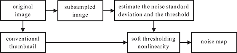
FIGURE 7.10
Multirate noise estimation flowchart.
7.5.1.2 Multirate Noise Estimation
The noise estimation method presented in Reference [4] also relies on wavelet-based soft thresholding [51]. Instead of a full wavelet transform, a single high-pass filtered signal is used to generate the noise. This signal is determined as
where g(σ) is a Gaussian filter with standard variation σ = 1. The soft threshold nonlinearity, as defined in Equation 7.11, is applied to the filtered signal. Then the noise map is given by
where the threshold τ is estimated from xh without performing wavelet transform, and thus differing from region-based noise estimation. Here, the noise estimate ρ corresponds to the high-resolution original image. According to Reference [52], subsampling the noise estimate ρ by a scaling factor t generates the noise map n at the thumbnail resolution with the same standard deviation. Therefore, the noise map n can be computed as
In this noise estimation algorithm, estimating ρ can be rather slow due to the high resolution of the original image. A fast version of this algorithm was developed in Reference [9] by exchanging the order of subsampling and noise generation. More specifically, multirate signal transformations [52] was used to estimate the noise at the low thumbnail resolution. Multirate noise estimation is feasible since there are enough pixels at the thumbnail resolution for the determination of the noise standard deviation. In addition, the soft threshold nonlinearity commutes with the subsampling operator. Due to these two facts, subsampling can be applied to the high-resolution image and the noise estimate is performed on the subsampled low-resolution image. Note that the threshold τ is estimated from the low-resolution image subsampled from the high-resolution image. Figure 7.10 illustrates the process of multirate noise estimation. Readers are referred to Reference [9] for a more detailed analysis of multirate noise estimation.
7.5.2 Noise Visualization
Visualizing noise is rather simple. As the noise is assumed to be additive to the ideal signal, the noise-preserved thumbnail is formed by adding the estimated noise map n to the thumbnail. Considering image blur, the noise visualization is performed after blur visualization as follows:
where the parameter mag controls the strength of noise to be visualized.
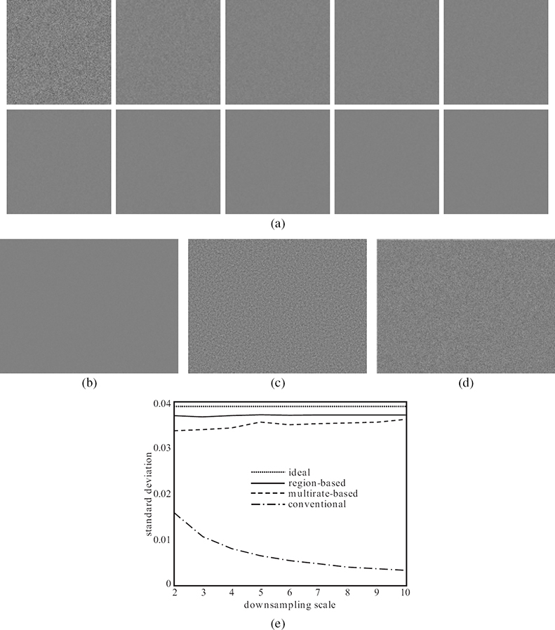
FIGURE 7.11
Evaluation of noise estimation: (a) 100 × 100 region at downsampling scales ranging from one to ten, with one corresponding to the original noise, (b) conventional thumbnail at the downsampling scale of ten, (c) regionbased thumbnail, (d) multirate estimation-based thumbnail, and (e) plots of standard deviation of pixel intensities against the downsampling scales.
7.5.3 Evaluation
A simulation using a noise image is conducted to evaluate the performance of the two noise estimation methods. To roughly simulate the observed noise in photographs [53], the noise image is generated by adding a Gaussian noise with the standard deviation σ = 10/255 = 0.392 to a gray image with constant values. In Figure 7.11a, the 2048 × 1536 noise image (with one patch shown in the left-top position) is downsampled by different subsampling factors. At each subsampling scale, a 100 × 100 region is cropped for illustration. It is obvious that increasing the subsampling scale reduces the strength of noise gradually. In the thumbnail of a resolution 205 × 154 shown in Figure 7.11b, the noise is almost invisible. The two noise estimation methods, with the outputs shown in Figures 7.11c and 7.11d, are applied at each downsampling scale to estimate the noise map. Figure 7.11e shows the results of the standard deviations for the estimated noise maps with respect to the subsampling factors. The conventional thumbnail has a decreased standard deviation. The decreasing slope verifies the observation that the larger the subsampling factor is, the less noisy the thumbnail appears. Both noise estimation methods, on the other hand, have nearly horizontal lines and quite close to the ideal curve. The results indicate that the two methods are able to preserve the noise standard deviations faithfully across scale.
7.6 Experimental Results
This section presents some experimental results and comparisons of perceptual thumbnail generation with the ability of highlighting blur and noise. All results reported here are produced using α = 1, β = 3.0, τ = 2.0, and γ = 1.5.
First, the experimental results on blur highlighting are reported. Note that a good blur highlighting algorithm should be able to reflect present blur and should not to introduce obvious blur when the picture is sharp. Figure 7.12 demonstrates a blurry picture due to camera shake. The conventional thumbnail with 423 × 317 pixels appears rather clear and sharp, although the magnified regions in the original high-resolution image with 2816 × 2112 pixels look blurry. Both gradient-based and scale-space-based blur estimation can reflect blur in the modulated thumbnails. Visual inspection of the corresponding blur maps reveals that both methods have effects around edge regions. The difference is that the gradient-based method visualizes blur around salient edges only, while the scale-space-based method is effective in most edges, including weak edges. In terms of visual experience, the scale-space-based method introduces larger blur that is thus more visible to viewers; however, it appears to produce block artifacts.
Now that the existing blur highlighting methods are effective for blurry pictures, their performance is exploited in the case of sharp pictures, for which the methods are expected to introduce as small blur as possible. Refer to Figures 7.13 and 7.14. The two highresolution pictures with 2048 × 1536 pixels are shot without motion blur or camera shake. One can see in the magnified image region that the edges are rather strong and sharp. Hence, the perceptual thumbnail at a resolution of 342 × 256 pixels should look similar to the conventional thumbnail, which is also sharp and clear. A close inspection of the thumbnails in Figures 7.13c, 7.13d, 7.14b, and 7.14c reveals that either method introduces some blur in the resulted thumbnails. From side-by-side comparisons, it can be observed that the gradient-based method suffers less from the unexpected blur, and the scale-space-based method may introduce obvious distracting blur in some regions.
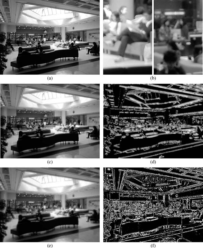
FIGURE 7.12 (See color insert.)
Highlighting blur in the thumbnail when the original image is blurred: (a) conventional thumbnail at a resolution of 423 × 317 pixels, (b) two magnified regions from the original image with 2816 × 2112 pixels, (c) perceptual thumbnail obtained using gradient-based blur estimation, (d) corresponding blur map, (e) perceptual thumbnail obtained using the scale-space-based blur estimation, and (f) corresponding blur map.
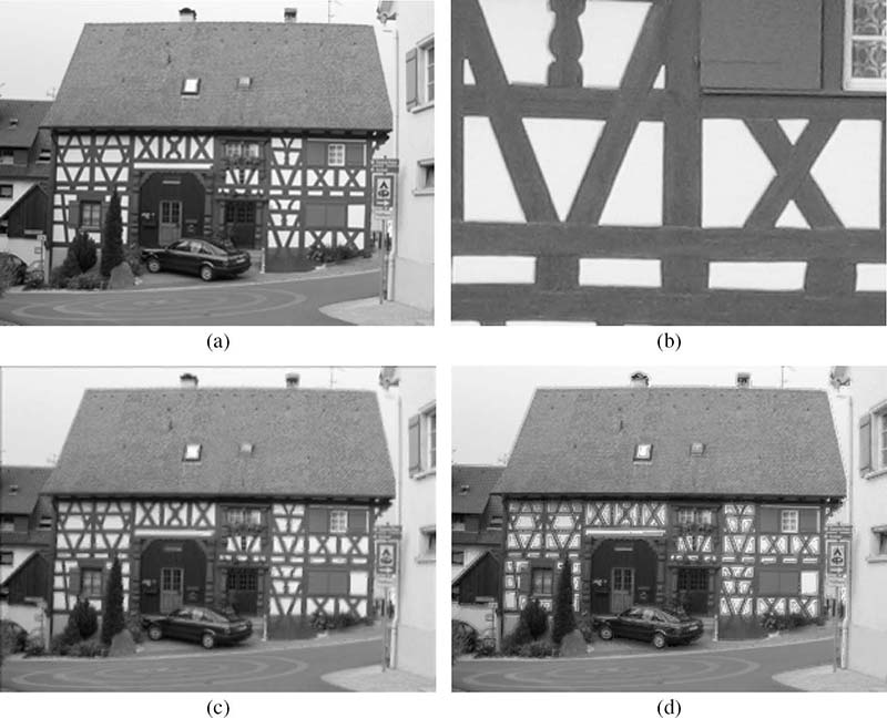
FIGURE 7.13 (See color insert.)
Highlighting blur in the thumbnail when the original image is sharp: (a) conventional thumbnail with 341 × 256 pixels, (b) magnified region from the original image with 2048 × 1536 pixels, (c) perceptual thumbnail via gradient-based blur estimation, and (d) perceptual thumbnail via scale-space-based blur estimation.
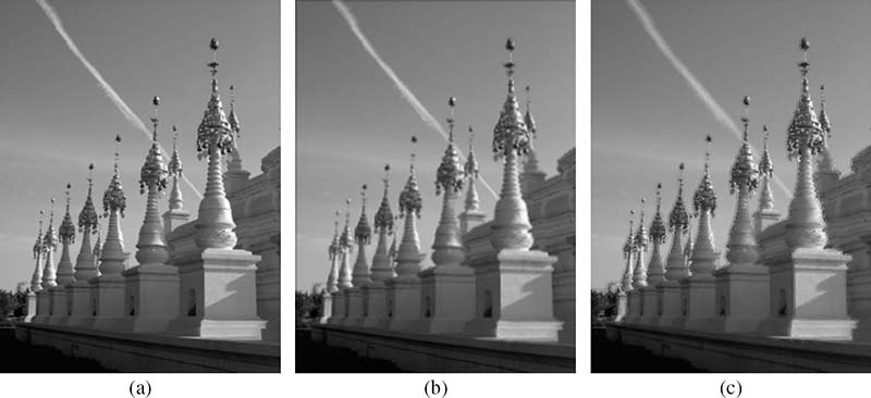
FIGURE 7.14 (See color insert.)
Highlighting blur in the thumbnail when the original image with 1536 χ 2048 pixels is sharp: (a) conventional thumbnail with 256 × 341 pixels, (b) perceptual thumbnail via gradient-based blur estimation, and (c) perceptual thumbnail via scale-space-based blur estimation.
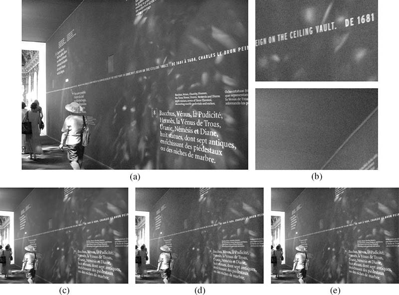
FIGURE 7.15
Highlighting noise in the thumbnail: (a) original noisy image, (b) two magnified regions from the original image, (c) conventional thumbnail, (d) perceptual thumbnail obtained using region-based noise estimation, and (e) perceptual thumbnail obtained using multirate noise estimation.
The following discusses the experimental results for noise highlighting. Similar to the requirements of blur highlighting methods, a good noise highlighting method shall be able to visualize image noise for noisy images, and not to introduce apparent noise for noise-free images. Figures 7.15 and 7.16 compare the conventional thumbnail and the perceptual thumbnail from region-based noise estimation and multirate noise estimation. The two high-resolution images (2272 × 1704 and 2048 × 1536 pixels) suffer from severe noise; however, such noise cannot be observed when viewing their conventional thumbnails. On the contrary, the two noise estimation methods are able to generate thumbnails that reflect noise in a similar way to the original high-resolution images.
In Figure 7.17, noise estimation is performed for a noise-free high-resolution image with 2048 × 1536 pixels. The perceptual thumbnail should be similar to the conventional thumbnail which looks clean. Comparing the results reveals that the thumbnail from region-based noise estimation is almost the same as the conventional thumbnail. The thumbnail from multirate noise estimation has details enhanced in texture-intensive regions. Here, both noise estimation methods used Equation 7.16 with the parameter mag = 2. A smaller value of this parameter can be used to reduce the level of detail enhancement.
Finally, Figure 7.18 shows an example that combines both blur highlighting and noise highlighting. The high-resolution image with 2048 × 1536 pixels suffers from image blur and noise that take effect in the entire image. The thumbnails generated by using bilinear, bicubic, and Lanczos filtering methods shown in Figures 7.18c to Figures 7.18e appear rather clean and clear; by viewing these thumbnails the user cannot tell that the highresolution image is noisy and blurry. This is not the case when the thumbnails are created by adding blur only according to the gradient-based and scale-space-based blur estimation methods. Comparing the resulted thumbnails with the conventional ones, image blur is reflected in the resulted thumbnails. The final thumbnails are generated by superimposing the estimated noise. As can be seen in Figures 7.18h and 7.18k, the perceptual thumbnails well reflect the blur and noise present in the high-resolution image.
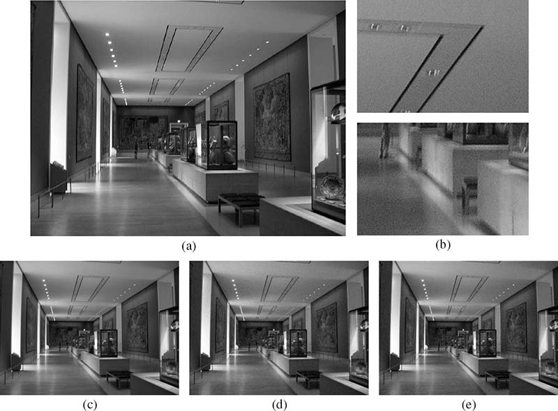
FIGURE 7.16
Highlighting noise in the thumbnail: (a) original noisy image, (b) two magnified regions from the original image, (c) conventional thumbnail, (d) thumbnail obtained using region-based noise estimation, and (e) thumbnail obtained using multirate noise estimation.
7.7 Conclusion
This chapter discussed perceptual thumbnail generation, a practical problem available in digital photography, image browsing, image searching, and web applications. Differing from the conventional image thumbnails, the perceptual thumbnails allows inspecting the image quality at the small thumbnail resolution. Perceptual thumbnails serve in an intuitive way by displaying the perception-related visual cues in the thumbnail resolution.
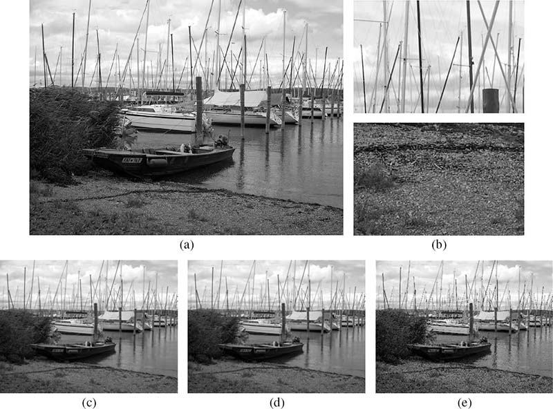
FIGURE 7.17
Highlighting noise in the thumbnail: (a) original noise-free image, (b) two magnified regions from the original image, (c) conventional thumbnail, (d) thumbnail obtained using region-based noise estimation, and (e) thumbnail obtained using multirate noise estimation.
Perceptual thumbnail generation is still a rather new problem in the field of computer vision and media computing. Existing methods mainly focus on two low-level visual cues, that is, blur and noise. Although blur and noise estimation and removal have been extensively studied, the goal of most techniques is to obtain the blur kernel and noise model and in turn to reconstruct the ideal image. Perceptual thumbnail generation does not have such strict requirements for blur and noise estimation. A rough and fast estimation is sufficient and necessary in this case. Existing techniques on perceptual thumbnail generation exploit how to assess the local spatial-varying blur strength and the noise in a fast way.
One potential future task for perceptual thumbnail generation is to highlight other visual cues, like the red-eye effect. There are many works on detecting and removal red-eye effects [36], [37]. However, visualizing red eyes in the thumbnail is not as straightforward as highlighting blur and noise. Superimposing the detected red eyes with the thumbnail may result in an unnatural preview. To highlight red eyes in the thumbnail, a possible solution is to mark its region in the thumbnail. For example, one may draw a red ellipse around the defected eyes. Image bloom is another phenomenon which is associated with similar problems, that is, how to effectively visualize it in thumbnails.
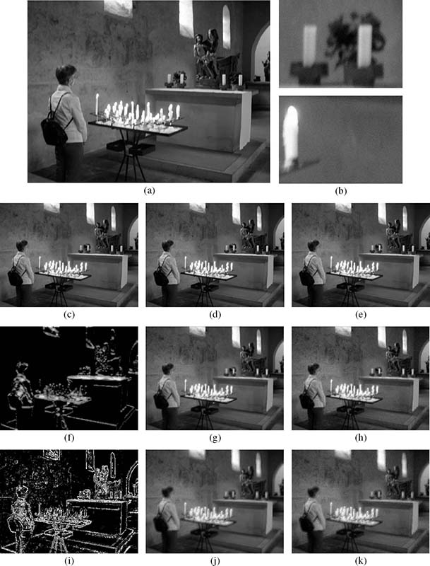
FIGURE 7.18 (See color insert.)
Highlighting blur and noise in the thumbnail: (a) original image with both blur and noise, (b) two magnified regions from the original image, (c) conventional thumbnails obtained using bilinear filtering, (d) conventional thumbnails obtained using bicubic filtering, (e) conventional thumbnails obtained using Lanczos filtering, (f) gradient-based estimation blur map, (g) perceptual thumbnail obtained using gradient-based blur estimation, (h) perceptual thumbnail obtained using gradient-based blur estimation and region-based noise estimation, (i) scale-space-based estimation blur map, (i) perceptual thumbnail obtained using scale-space-based blur estimation, and (k) perceptual thumbnail obtained using scale-space-based blur estimation and multirate noise estimation.
Acknowledgment
This research is partially supported by project #MMT-p2-11 of the Shun Hing Institute of Advanced Engineering, The Chinese University of Hong Kong.
References
[1] C. Burton, J. Johnston, and E. Sonenberg, “Case study: An empirical investigation of thumbnail image recognition,” in Proceedings of the IEEE Symposium on Information Visualization, Atlanta, Georgia, USA, October 1995, pp. 115–121.
[2] K. Berkner, E. Schwartz, and C. Marle, “Smart nails: Display- and image-dependent thumbnails,” in Proceedings of the SPIE Conference on Document Recognition and Retrieval, San Jose, CA, USA, December 2003, pp. 54–65.
[3] A. Woodruff, A. Faulring, R. Rosenholtz, J. Morrison, and P. Pirolli, “Using thumbnails to search the web,” in Proceedings of the ACM Conference on Human Factors in Computing Systems, Seattle, WA, USA, March 2001, pp. 198–205.
[4] R. Samadani, S.H. Lim, and D. Tretter, “Representative image thumbnails for good browsing,” in Proceedings of the IEEE International Conference on Image Processing, San Antonio, TX, USA, September 2007, vol. 2, pp. 193–196.
[5] L. Wan, W. Feng, Z.C. Lin, T.T. Wong, and Z.Q. Liu, “Perceptual image preview,” Multimedia Systems, vol. 14, no. 4, pp. 195–204, September 2008.
[6] W. Burger and M.J. Burge, Principles of Digital Image Processing: Core Algorithms. London, UK: Springer, 2009.
[7] A. Muñoz, T. Blu, and M. Unser, “Least-squares image resizing using finite differences,” IEEE Transactions on Image Processing, vol. 10, no. 9, pp. 1365–1378, September 2001.
[8] L.Q. Chen, X. Xie, X. Fan, W.Y. Ma, H.J. Zhang, and H.Q. Zhou, “A visual attention model for adapting images on small displays,” ACM Multimedia Systems Journal, vol. 9, no. 4, pp. 353–364, October 2003.
[9] R. Samadani, T.A. Mauer, D.M. Berfanger, and J.H. Clark, “Image thumbnails that represent blur and noise,” IEEE Transactions on Image Processing, vol. 19, no. 2, pp. 363–373, Feburary 2010.
[10] R.G. Keys, “Cubic convolution interpolation for digital image processing,” IEEE Transaction on Acoustics, Speech, and Signal Processing, vol. 29, no. 6, pp. 1153–1160, December 1981.
[11] M. Unser, “Splines: A perfect fit for signal and image processing,” IEEE Transaction on Signal Processing, vol. 16, no. 6, pp. 22–38, November 1999.
[12] E.H.W. Meijering, W.J. Niessen, and M.A. Viergever, “Piecewise polynomial kernels for image interpolation: A generalization of cubic convolution,” in Proceedings of the IEEE International Conference of Image Processing, Kobe, Japan, October 1999, vol. 3, pp. 647–651.
[13] X. Li, Edge Directed Statistical Inference with Applications to Image Processing. PhD thesis, Princeton University, Princeton, NJ, USA, 2000.
[14] B. Suh, H. Ling, B.B. Bederson, and D.W. Jacobs, “Automatic thumbnail cropping and its effectiveness,” in Proceedings of the 16th Annual ACM Symposium on User Interface Software and Technology, Vancouver, Canada, November 2003, pp. 95–104.
[15] S. Avidan and A. Shamir, “Seam carving for content-aware image resizing,” ACM Transaction on Graphics, vol. 26, no. 3, pp. 10:1–9, July 2007.
[16] Y.S. Wang, C.L. Tai, O. Sorkine, and T.Y. Lee, “Optimized scale-and-stretch for image resizing,” ACM Transactions on Graphics, vol. 27, no. 5, pp. 118:1–8, December 2008.
[17] P. Thevenaz, T. Blu, and M. Unser, Image Interpolation and Resampling. New York, USA: Academic Press, 2000.
[18] D.P. Mitchell and A.N. Netravali, “Reconstruction filters in computer graphics,” SIGGRAPH Computer Graphics, vol. 22, no. 4, pp. 221–228, August 1988.
[19] N. Greene and P. Heckbert, “Creating raster omnimax images from multiple perspective views using the elliptical weighted average filter,” IEEE Computer Graphics and Applications, vol. 6, no. 6, pp. 21–27, June 1986.
[20] P. Heckbert, Fundamentals of Texture Mapping and Image Warping. Master’s thesis, University of California, Berkeley, CA, USA, 1989.
[21] J. McCormack, R. Perry, K.I. Farkas, and N.P. Jouppi, “Feline: Fast elliptical lines for anisotropic texture mapping,” in Proceedings of the 26th Annual Conference on Computer Graphics and Interactive Techniques, Los Angeles, CA, USA, August 1999, pp. 243–250.
[22] X. Li and M. Orchard, “New edge-directed interpolation,” IEEE Transactions on Image Processing, vol. 10, no. 10, pp. 1521–1527, October 2001.
[23] D. Muresan and T. Parks, “Adaptively quadratic (AQUA) image interpolation,” IEEE Transactions on Image Processing, vol. 13, no. 5, pp. 690–698, May 2004.
[24] L. Zhang and X. Wu, “An edge-guided image interpolation algorithm via directional filtering and data fusion,” IEEE Transactions on Image Processing, vol. 15, no. 8, pp. 2226–2238, August 2006.
[25] R. Fattal, “Image upsampling via imposed edge statistics,” ACM Transactions on Graphics, vol. 26, no. 3, pp. 95:1–8, July 2007.
[26] V.R. Setlur, Optimizing Computer Imagery for More Effective Visual Communication. PhD thesis, Northwestern University, Evanston, IL, USA, 2005.
[27] Y. Pritch, E. Kav-Venaki, and S. Peleg, “Shift-map image editing,” in Proceedings of the International Conference on Computer Vision, Kyoto, Japan, September 2009, pp. 151–158.
[28] P. Krahenbuhl, M. Lang, A. Hornung, and M. Gross, “A system for retargeting of streaming video,” ACM Transactions on Graphics, vol. 28, no. 5, pp. 126:1–126:10, December 2009.
[29] M. Rubinstein, A. Shamir, and S. Avidan, “Multi-operator media retargeting,” ACM Transactions on Graphics, vol. 28, no. 3, pp. 23:1–11, July 2009.
[30] M. Rubinstein, D. Gutierrez, O. Sorkine, and A. Shamir, “A comparative study of image retargeting,” ACM Transactions on Graphics, vol. 29, no. 6, pp. 160:1–10, December 2010.
[31] H. Lam and P. Baudisch, “Summary thumbnails: Readable overviews for small screen web browsers,” in Proceedings of the SIGCHI Conference on Human Factors in Computing Systems, Portland, OR, USA, April 2005, pp. 681–690.
[32] A. Cockburn, C. Gutwin, and J. Alexander, “Faster document navigation with space-filling thumbnails,” in Proceedings of the SIGCHI Conference on Human Factors in Computing Systems, Montreal, QC, Canada, April 2006, pp. 1–10.
[33] S. Baluja, “Browsing on small screens: Recasting web-page segmentation into an efficient machine learning framework,” in Proceedings of the 15th International Conference on World Wide Web, Edinburgh, Scotland, May 2006, pp. 33–42.
[34] A. Wrotniak, “Noise in digital cameras.” Available online, http://www.wrotniak.net/photo/tech/noise.html, 2008.
[35] Y. Ke, X. Tang, and F. Jing, “The design of high-level features for photo quality assessment,” in Proceedings of the IEEE Conference on Computer Vision and Pattern Recognition, New York, USA, June 2006, vol. 1, pp. 419–426.
[36] L. Zhang, Y. Sun, M. Li, and H. Zhang, “Automated red-eye detection and correction in digital photographs,” in Proceedings of the International Conference on Image Processing, Singapore, October 2004, vol. 4, pp. 2363–2366.
[37] F. Volken, J. Terrier, and P. Vandewalle, “Automatic red-eye removal based on sclera and skin tone detection,” in Proceedings of the IS&T Third European Conference on Color in Graphics, Imaging and Vision, Sydney, Australia, July 2006, pp. 359–364.
[38] N. El-Yamany, Faithful Quality Representation of High-Resolution Imagess at Low Resolutions. PhD thesis, Southern Methodist University, Dallas, TX, USA, 2010.
[39] M. Trentacoste, R. Mantiuk, and W. Heidrich, “Quality-preserving image downsizing,” in Proceedings of the 3rd ACM Conference and Ehibition on Computer Graphics and Interactive Techniques in Asia, Seoul, Korea, December 2010, p. 74.
[40] D. Kundur and D. Hatzinakos, “Blind image deconvolution,” IEEE Signal Processing Magazine, vol. 13, no. 3, pp. 43–64, May 1996.
[41] Q. Shan, J. Jia, and A. Agarwala, “High-quality motion deblurring from a single image,” ACM Transactions on Graphics, vol. 27, no. 3, pp. 73:1–10, August 2008.
[42] N. Joshi, C.L. Zitnick, R. Szeliski, and D.J. Kriegman, “Image deblurring and denoising using color priors,” in Proceedings of the IEEE Conference on Computer Vision and Pattern Recognition, Miami, FL, USA, June 2009, pp. 1550–1557.
[43] A.S. Wilsky, “Multiresolution Markov models for signal and image processing,” Proceedings of the IEEE, vol. 90, no. 8, pp. 1396–1458, August 2002.
[44] M. Zhang and B.K. Gunturk, “Multiresolution bilateral filtering for image denoising,” IEEE Transactions on Image Processing, vol. 17, no. 12, pp. 2324–2333, December 2008.
[45] P. Marziliano, F. Dufaux, S. Winkler, and T. Ebrahimi, “A no-reference perceptual blur metric,” in Proceedings of the International Conference on Image Processing, Lausanne, Switzerland, December 2002, vol. 3, pp. 57–60.
[46] J. Caviedes and F. Oberti, “A new sharpness metric based on local kurtosis, edge and energy information,” Signal Processing: Image Communication, vol. 19, no. 2, pp. 147–161, February 2004.
[47] R. Ferzli and L. Karam, “No-reference objective wavelet based noise immune image sharpness metric,” in Proceedings of the IEEE International Conference on Image Processing, Genoa, Italy, September 2005, vol. 1, pp. 405–408.
[48] M.C. Chiang and T.E. Boult, “Local blur estimation and super-resolution,” in Proceedings of the Conference on Computer Vision and Pattern Recognition, June 1997, pp. 821–826.
[49] J.H. Elder and S.W. Zucker, “Local scale control for edge detection and blur estimation,” IEEE Transaction on Pattern Analysis and Machine Intelligience, vol. 20, no. 7, pp. 699–716, July 1998.
[50] S. Bae and F. Durand, “Defocus magnification,” Computer Graphics Forum, vol. 26, no. 3, pp. 571–579, September 2007.
[51] D.L. Donoho, “De-noising by soft-thresholding,” IEEE Transactions on Information Theory, vol. 41, no. 3, pp. 613–627, May 1995.
[52] P. Vaidyanathan, Multirate Systems and Filter Banks. Upper Saddle River, NJ, USA: Prentice Hall, 1993.
[53] S.H. Lim, “Characterization of noise in digital photographs for image processing,” Proceedings of SPIE, vol. 6069, pp. 219–228, April 2006.