6 Joint White Balancing and Color Enhancement

Despite recent advances in digital color imaging [1], [2], producing digital photographs that are faithful representations of the original visual scene remains still challenging due to a number of constraints under which digital cameras operate. In particular, differences in characteristics between image acquisition systems and the human visual system constitute an underlying problem in digital color imaging. Digital cameras typically use various color filters [3], [4], [5] to reduce the available color information to the light of certain wavelengths, which is then sampled by the image sensor, such as a charge-coupled device (CCD) [6], [7] or a complementary metal oxide semiconductor (CMOS) sensor [8], [9]. Unfortunately, achieving a precise digital representation of the visual scene is still not quite possible and extensive processing [10], [11], [12] of acquired data is needed to reduce an impact of shortcomings of the imaging system.

Images

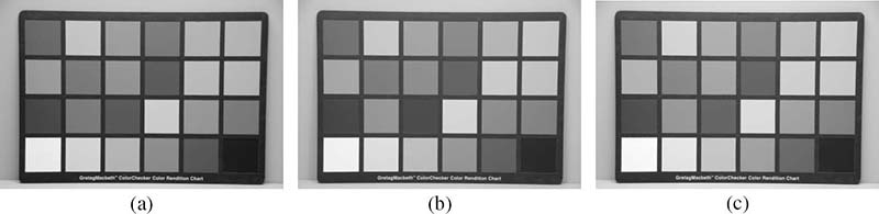
FIGURE 6.1 (See color insert.)
The Macbeth color checker taken under the (a) daylight, (b) tungsten, and (c) fluorescent illumination.

For example, as shown in Figure 6.1, the coloration of captured images often appears different from the visual scene, depending on the illumination under which the image is taken. Although various light sources usually differ in their spectral characteristics [13], [14], [15], the human visual system is capable of discounting the dominant color of the environment, usually attributed to the color of a light source. This ability ensures the approximately constant appearance of an object for different illuminants [16], [17], [18], [19] and is known under the name of chromatic adaptation. However, digital cameras have to rely on the image processing methods, termed as white balancing [20], [21], [22], [23], to produce images with appearances close to what is observed by the humans. Some cameras use a sensor to measure the illumination of the scene; an alternative is to estimate the scene illuminant by analyzing the captured image data. In either case, fixed parameters are typically used for the whole image to perform the adjustment for the scene illuminant.

This chapter presents a framework [24], [25] that enhances the white balancing process by combining the global and local spectral characteristics of the captured image. This framework takes advantage of the refined color modeling and manipulation concepts in order to adjust the acquired color information adaptively in each pixel location. The presented design methodology is reasonably simple, highly flexible, and provides numerous attractive solutions that can produce visually pleasing images with enhanced coloration and improved color contrast.

To facilitate the subsequent discussions, Section 6.2 presents the fundamentals of color vision and digital color imaging, including the adaptation mechanisms of the human visual system, basic numerical representations of color signals, and various practical color modeling concepts. Section 6.3 focuses on the white balancing basics and briefly surveys several popular methods. Section 6.4 introduces the framework for joint white balancing and color enhancement. Motivation and design characteristics are discussed in detail, and some example solutions designed within this framework are showcased in different application scenarios and analyzed in terms of their computational complexity. Section 6.5 describes methods that are commonly used for color image quality evaluation and quantitative manipulation. Finally, conclusions are drawn in Section 6.6.

Images

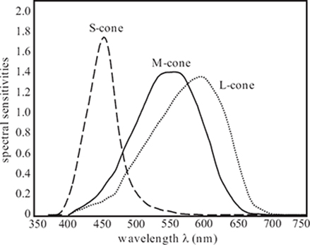
FIGURE 6.2
Estimated effective sensitivities of the cones. Peak sensitivities correspond to the light with wavelengths of approximately 420 nm for S-cones, 534 nm for M-cones, and 564 nm for L-cones.

6.2 Color Vision Basics

Color is a psycho-physiological sensation [26] used by the observers to sense the environment and understand its visual semantics. It is interpreted as a perceptual result of the light interacting with the spectral sensitivities of the photoreceptors.

Visible light is referred to as electromagnetic radiation with wavelengths λ ranging from about 390 to 750 nanometers (nm). This small portion of the electromagnetic spectrum is referred to as the visible spectrum. Different colors correspond to electromagnetic waves of different wavelengths; the sensation of violet appears at 380 to 450 nm, blue at 450 to 475 nm, cyan at 476 to 495 nm, green at 526 to 606 nm, yellow at 570 to 590 nm, orange at 590 to 620 nm, and red at 620 to 750 nm. The region below 390 nm is called ultra-violet, the region above 750 nm is called infra-red.

The human visual system is based on two types of photoreceptors localized on the retina of the eye; the rods sensitive to light, and the cones sensitive to color [16]. The rods are crucial in scotopic vision, which refers to vision in low light conditions where no color is usually seen and only shades of gray can be perceived. In photopic vision, which refers to vision in typical light conditions, the rods become saturated and thus the perception mechanism completely relies on less-sensitive cones. Both rods and cones contribute to vision for certain illumination levels, creating thus gradual changes from scotopic to photopic vision.

It is estimated that humans are capable of resolving about 10 million color sensations [20]. The perception of color depends on the response of three types of cones, commonly called S-, M-, and L-cones for their respective sensitivity to short, middle, and long wavelengths. The different sensitivity of each type of cones is attributed to the spectral absorption characteristics of their photosensitive pigments. Two spectrally different lights that have the same L-, M-, and S-cone responses give the same color sensation; this phenomenon is termed as metamers [16], [17].

Images

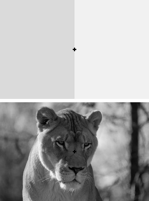
FIGURE 6.3 (See color insert.)
Chromatic adaptation. Stare for twenty seconds at the cross in the center of the top picture. Then focus on the cross in the bottom picture; the color casts should disappear and the image should look normal.

6.2.1 Adaptation Mechanisms of the Human Visual System

The human visual system is capable of changing its sensitivity in order to adapt to prevailing lighting conditions (Figure 6.3), thus maximizing its ability to extract information from the actual environment. It operates over a very large range of illumination, although the range of light that can be processed and interpreted simultaneously is rather limited [17]. Some quick changes are achieved through the dilation and constriction of the pupil in the eye, thus directly controlling the amount of light that can enter the eye [18]. The actual sensitivity changes with the response of the receptive cells on the retina of the eye. This is a slower process and may take a few minutes until the visual system is fully adjusted to the actual lighting conditions. Temporal adaptation and steady-state adaptation refer, respectively, to the performance of the human visual system during the adaptation process and in the situations when this process has been completed [17].

Light and dark adaptation [17], [18] are the two special cases which refer to the process of adjusting for the transition from a bright environment to a dark environment and from a fully adapted dark environment to a bright environment, respectively. Transient adaptation [19] refers to the situations typical for high-contrast visual environments, where the eye has to adapt from low to high light levels and back in short intervals. This readaptation from one luminous background to another reduces the equivalent (perceived) contrast; this loss can be expressed using the so-called transient adaptation factor.

Chromatic adaptation [17], [18] characterizes the ability of the human visual system to discount the dominant color of the environment, usually attributed to the color of a light source, and thus approximately preserve the appearance of an object under various illuminants. Different types of the receptive cells in the eye are sensitive to different bands in the visible spectrum. If the actual lighting situation has a different color temperature compared to the previous lighting conditions, the cells responsible for sensing the light in a band with increased (or reduced) amount of light relative to the total amount of light from different bands, will reduce (or increase) their sensitivity relative to the sensitivity of the other cells. This effectively performs automatic white balancing of the human visual system. Assuming that chromatic adaptation is an independent gain regulation of the three sensors in the human visual system, these relations of the spectral sensitivities can be expressed as [17]:

$\begin{matrix} l_{2} (λ) = k_{l} l_{1} (λ), & m_{2} (λ) = k_{m} m_{1} (λ), & s_{2} (λ) = k_{s} s_{1} (λ) \end{matrix}, (6.1)$

where l₁(λ), m₁(λ), and s₁(λ) denote the the spectral sensitivities of the three receptors at one state of adaptation and l₂(λ), m₂(λ), and s₂(λ) for a different state. The coefficients k_l, k_m, and k_s are inversely related to the relative strengths of activation.

Chromatic adaptation models, such as the one presented above, are essential in describing the appearance of a stimulus and predicting whether two stimuli will match if viewed under disparate lighting conditions where only the color of the lighting has changed. Various computational models of chromatic adaptation are surveyed in References [17] and [18].

6.2.2 Numeral Representation of Color

Color cannot be specified without an observer and therefore it is not an inherent feature of an object. The color stimulus S (λ) depends on both the illumination I (λ) and the object reflectance R(λ); this relationship can be expressed as follows [20], [27]:

$\begin{array}{l} S (λ) & = & I (λ) R (λ), \\ = & (\sum_{j = 1}^{m} α_{j} I_{j} (λ)) (\sum_{k = 1}^{m} β_{k} R_{k} (λ)), \\ = & \sum_{j = 1}^{m} \sum_{k = 1}^{n} α_{j} β_{k} I_{j} (λ) R_{k} (λ), \end{array} (6.2)$

where I_j (λ) and R_k(λ) terms denote known basis functions. Given any object, it is possible to theoretically manipulate the illumination so that it produces any desired color stimulus.

Figure 6.4 shows the spectral power distribution of sunlight, tungsten, and fluorescent illuminations. The effect of these illumination types on the appearance of color is demonstrated in Figure 6.1.

Images

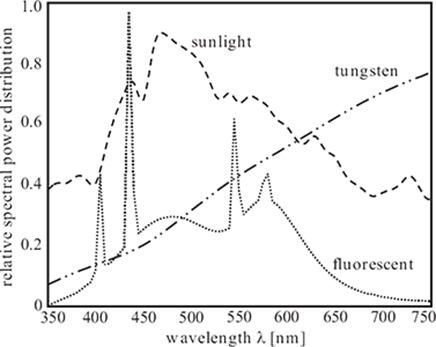
FIGURE 6.4
Spectral power distribution of common illuminations.

When an object with stimulus S(λ) is observed, each of the three cone types responds to the stimulus by summing up the reaction at all wavelengths [20]:

$\begin{array}{l} X & = & \int_{390}^{750} l (λ) I (λ) R (λ) d λ, \\ Y & = & \int_{390}^{750} m (λ) I (λ) R (λ) d λ, \\ Z & = & \int_{390}^{750} s (λ) I (λ) R (λ) d λ, \end{array} (6.3)$

where l(λ), m(λ), and s(λ) denote the spectral sensitivities of the L-, M-, and S-cones depicted in Figure 6.2.

Since three signals are generated based on the extent to which each type of cones is stimulated, any visible color can be numerically represented using three numbers called tristimulus values as a three-component vector within a three-dimensional coordinate system with color primaries lying on its axes [28]. The set of all such vectors constitutes the color space.

Numerous color spaces and the corresponding conversion formulas have been designed to convert the color data from one space to some other space, which is more suitable for completing a given task and/or addresses various design, performance, implementation, and application aspects of color image processing. The following discusses two representations relevant to the scope of this chapters.

6.2.2.1 Standardized Representations

The Commission Internationale de l’Éclairage (CIE) introduced the standardized CIE-RGB and CIÉ-XYZ color spaces. The well-known Red-Green-Blue (RGB) space was derived based on color matching experiments, aimed at finding a match between a color obtained through an additive mixture of color primaries and a color sensation [29]. Its standardized version [30] is used in most of today’s image acquisition and display devices. It provides a reasonable resolution, range, depth, and stability of color reproduction while being efficiently implementable on various hardware platforms.

Images

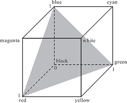
FIGURE 6.5
RGB color space.

The RGB color space can be derived from the XYZ space, which is another standardized space. Since the XYZ space is device independent, it is thus very useful in situations where consistent color representation across devices with different characteristics is required. Al-though the CIE-XYZ color space is rarely used in image processing applications, other color spaces can be derived from it through mathematical transforms.

A relationship between these two spaces can be expressed as follows [28], [31]:

$[\begin{matrix} X \\ Y \\ Z \end{matrix}] = [\begin{matrix} 0.49 & 0.31 & 0.20 \\ 0.17697 & 0.81240 & 0.01063 \\ 0 & 0.01 & 0.99 \end{matrix}] [\begin{matrix} R \\ G \\ B \end{matrix}] (6.4)$

where the Y component corresponds to the luminance, whereas X and Z do not correspond to any perceptual attributes.

The RGB space is additive; as shown in Figure 6.5, any color can be obtained by combining the three primaries through their weighted contributions [29]. Equal contributions of all three primaries give a shadow of gray. The two extremes of gray are black and white, which correspond, respectively, to no contribution and the maximum contributions of the color primaries. When one primary contributes greatly, the resulting color is a shade of that dominant primary. Any pure secondary color is formed by maximum contributions of two primary colors: cyan is obtained using green and blue, magenta using red and blue, and yellow using red and green. When two primaries contribute greatly, the result is a shade of the corresponding secondary color.

The RGB space models the output of physical devices, and therefore it is considered device dependent. To consistently detect or reproduce the same RGB color vector, some form of color management is usually required. This relates to the specification of the white point, gamma correction curve, dynamic range, and viewing conditions [32]. Given an XYZ color vector with components ranging from zero to one and the reference white being the same as that of the RGB system, the conversion to sRGB values starts as follows:

Images

FIGURE 6.6
Lab / Luv color space.

$[\begin{matrix} R \\ G \\ B \end{matrix}] = [\begin{matrix} 3.2410 & - 1.5374 & - 0.4986 \\ - 0.9692 & 1.8760 & 0.0416 \\ 0.0556 & - 0.2040 & 1.0570 \end{matrix}] [\begin{matrix} X \\ Y \\ Z \end{matrix}] (6.5)$

To avoid values outside the nominal range, which are usually not supported in RGB encoding, both negative values and values exceeding one are clipped to zero and one, respectively. This step is followed by gamma correction:

$f (τ) = {\begin{array}{l} 1.055 τ^{1 / 2.4} - 0.055 & if τ > 0.00304, \\ 12.92 τ & otherwise, \end{array} (6.6)$

where τ denotes the uncorrected color component. Finally, gamma-corrected components f(R), f(G), and f(B) are multiplied by 255 to obtain their corresponding values in standard eight bits per channel encoding.

6.2.2.2 Perceptual Representations

Perceptually uniform CIE u, v, CIE-Luv, and CIE-Lab representations are derived from XYZ values. In the case of CIE u and v values, the conversion formulas

$\begin{matrix} u = \frac{4 X}{X + 15 Y + 3 Z}, & v = \frac{9 Y}{X + 15 Y + 3 Z} \end{matrix} (6.7)$

can be used to form a chromaticity diagram that corresponds reasonably well to the characteristics of human visual perception [33].

Converting the data from CIE-XYZ to CIE-Luv and CIE-Lab color spaces [31] requires a reference point in order to account for adaptive characteristics of the human visual system [29]. Denoting this point as [X_n, Y_n, Z_n] of the reference white under the reference illumination, the CIE-Lab values are calculated as

$\begin{array}{l} L^{*} = 116 f (Y / Y_{n}) - 16, \\ a^{*} = 500 (f (X / X_{n}) - f (Y / Y_{n})), \\ b^{*} = 200 (f (Y / Y_{n}) - f (Z / Z_{n})), \end{array} (6.8)$

whereas the CIE-Luv values are obtained as follows:

$\begin{array}{l} L^{*} = 116 f (Y / Y_{n}) - 16, \\ u^{*} = 13 L^{*} (u - u_{n}), \\ v^{*} = 13 L^{*} (v - v_{n}), \end{array} (6.9)$

where u_n = 4X_n/(X_n + 15Y_n + 3Z_n) and v_n = 9Y_n/(X_n + 15Y_n + 3Z_n) correspond to the reference point [X_n, Y_n, Z_n]. The terms u and v, calculated using Equation 6.7, correspond to the color vector [X, Y, Z] under consideration. Since the human visual system exhibits different characteristics in normal illumination and low light levels, f(·) is defined as follows [31]:

$f (γ) = {\begin{array}{l} γ^{1 / 3} & if γ >0 .008856, \\ 7.787 γ + 16 / 116 & otherwise . \end{array} (6.10)$

Figure 6.6 depicts the perceptual color space representation. The component L^*, ranging from zero (black) to 100 (white), represents the lightness of a color vector. All other components describe color; neutral or near neutral colors corresponds to zero or close to zero values of u^* and v^*, or a^* and b^*. Following the characteristics of opponent color spaces [34], u^* and a^* coordinates represent the difference between red and green, whereas v^* and b^* coordinates represent the difference between yellow and blue.

Unlike the CIE-XYZ color space, which is perceptually highly nonuniform, the CIE-Luv and CIE-Lab color spaces are suitable for quantitative manipulations involving color perception since equal Euclidean distances or mean square errors expressed in these two spaces equate to equal perceptual differences [35]. The CIE-Lab model also finds its application in color management [36], whereas the CIE-Luv model can assist in the registration of color differences experienced with lighting and displays [33].

6.2.3 Color Image Representation

An RGB color image x with K₁ rows and K₂ columns represents a two-dimensional matrix of three-component samples x_(r,s) = [x_(r,s)1, x_(r,s)2, x_(r,s)3] occupying the spatial location (r, s), with r = 1,2, …, K₁ and s = 1,2, …, K₂ denoting the row and column coordinates. In the color vector x_(rs), the terms x_(rs)1, x_(r,s)2, and x_(r,s)3 denote the R, G, and B component, respectively. In standard eight-bit RGB representation, these components can range from 0 to 255. The large value of x_(r,s)k, for k = 1,2,3, indicates high contribution of the kth primary in the color vector x_(rs). The process of displaying an image creates a graphical representation of the data matrix where the pixel values represent particular colors.

Each color vector x_(r,s) is uniquely defined by its magnitude

$\sqrt{x^{2}_{(r, s) 1} + x^{2}_{(r, s) 2} + x^{2}_{(r, s) 3}} (6.11)$

and direction

$x_{(r, s)} \sqrt{x^{2}_{(r, s) 1} + x^{2}_{(r, s) 2} + x^{2}_{(r, s) 3},} (6.12)$

which indirectly indicate luminance and chrominance properties of RGB colors, and thus are important for human perception [37]. Note that the magnitude represents a scalar value, whereas the direction, as defined above, is a vector. Since the components of this vector are normalized, such vectors form the unit sphere in the vector space.

Images

FIGURE 6.7
Luminance representation of the images shown in Figure 6.1 for the (a) daylight, (b) tungsten, and (c) fluorescent illumination.

Images

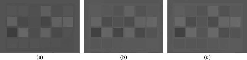
FIGURE 6.8 (See color insert.)
Chrominance representation of the images shown in Figure 6.1 for the (a) daylight, (b) tungsten, and (c) fluorescent illumination.

In practice, the luminance value L_(r,s) of the color vector x_(rs) is usually obtained as follows:

$L_{(r, s)} = 0.299 x_{(r, s) 1} + 0.587 x_{(r, s) 2} + 0.114 x_{(r, s) 3} . (6.13)$

The weights assigned to individual color channels reflect the perceptual contributions of each color band to the luminance response of the human visual system [16].

The chrominance properties of color pixels are often expressed as the point on the triangle, which intersects the RGB color primaries in their maximum value. The coordinates of this point are obtained as follows [38]:

$\frac{x_{(r, s) k}}{x_{(r, s) 1} + x_{(r, s) 2} + x_{(r, s) 3}}, for k = 1, 2, 3, (6.14)$

and their sum is equal to unity. Both above vector formulations of the chrominance represent the parametrization of the chromaticity space, where each chrominance line is entirely determined by its intersection point with the chromaticity sphere or chromaticity triangle in the three-dimensional vector space.

Figures 6.7 and 6.8, generated using Equations 6.13 and 6.14, respectively, show the luminance and chrominance representations of the images presented in Figure 6.1. As it can be seen, changing the illumination of the scene has a significant impact on the camera response, altering both the luminance and chrominance characteristics of the captured images.

6.2.4 Color Modeling

Any of the above definitions can be used to determine whether the two color vectors will appear similar to the observer under some viewing conditions. By looking at this problem from the other side, various color vectors matching the characteristics of the reference color vector can be derived based on some predetermined criterion. For example, simple but yet powerful color modeling concepts follow the observation that natural images consist of small regions that exhibit similar color characteristics. Since this is definitely the case of color chromaticity, which relates to the direction of the color vectors in the vector space, it is reasonable to assume that two color vectors x_(rs) and x_(i,j) have the same chromaticity characteristics if they are collinear in the RGB color space. Based on the definition of dot product x_(r,s). x_(i,j) = ||x_(r,s)||||x_(i,j)|| cos (〈x_(r,s), x_(i,j)〉), where ||x_(.,.)|| denotes the length of x_(,.,) and 〈x_(r,s), x_{(i, j)}〉 denotes the angle between three-component color vectors x_(r,s) and x_(i,j), the following can be derived [39]:

$〈 x_{(r, s)}, x_{(i, j)} 〉 = 0 \Leftrightarrow \frac{\sum_{k = 1}^{3} x_{(r, s) k} x_{(i, j) k}}{\sqrt{\sum_{k = 1}^{3} x_{(r, s) k}^{2}} \sqrt{\sum_{k = 1}^{3} x_{(i, j) k}^{2}}} = 1. (6.15)$

The above concept can be extended by incorporating the magnitude information into the modeling assumption. Using color vectors x_{(i, j)} and x_(r,s) as inputs, the underlying modeling principle of identical color chromaticity enforces that their linearly shifted variants [x_(r,s) + γI and [x_(i,j) + γI are collinear vectors:

$〈 x_{(r, s)} + γ I, x_{(i, j)} + γ I 〉 = 0 \Leftrightarrow \frac{\sum_{k = 1}^{3} (x_{(r, s) k} + γ) (x_{(i, j) k} + γ)}{\sqrt{\sum_{k = 1}^{3} {(x_{(r, s) k} + γ)}^{2}} \sqrt{\sum_{k = 1}^{3} {(x_{(i, j) k} + γ)}^{2}}} = 1. (6.16)$

where I is a unity vector of proper dimensions and x_(.,.)k + γ is the kth component of the linearly shifted vector [x_(.,.) + γI] = [x_(.,.)1 + γ, x_(.,.)2 + γ, x_(.,.)3 + γ]. A number of solutions can be obtained by modifying the value of γ, which is a design parameter that controls the influence of both the directional and the magnitude characteristics.

By reducing the dimensionality of the vectors to two components, some popular color correlation-based models can be obtained, such as the normalized color-ratio model [40]:

$\frac{x_{(r, s) k} + γ}{x_{(i, j) k} + γ} = \frac{x_{(r, s) 2} + γ}{x_{(i, j) 2} + γ}, (6.17)$

or the color-ratio model [41] given by

$\frac{x_{(r, s) k}}{x_{(i, j) k}} = \frac{x_{(r, s) 2}}{x_{(i, j) 2}}, (6.18)$

which both enforce hue uniformity. Another modeling option is to imply uniform image intensity by constraining the component-wise magnitude differences, as implemented by the color-difference model [42]:

$x_{(r, s) k} - x_{(i, j) k} = x_{(r, s) k} - x_{(i, j) / 2} . (6.19)$

The above modeling concepts have proved to be very valuable in various image processing tasks, such as demosaicking, denoising, and interpolation. It will be shown later that similar concepts can also be used to enhance the white balancing process.

Images

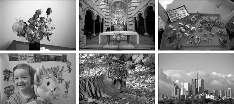
FIGURE 6.9 (See color insert.)
Examples of the images taken in different lighting conditions without applying white balancing.

6.3 White Balancing

As previously noted, the humans observe the approximately constant appearance of an object in different lighting conditions. This phenomenon of chromatic adaptation, also termed as color constancy, suggests that the human visual system transforms recorded stimuli into representations of the scene reflectance that are largely independent of the scene illuminant [16].

Automatic white balancing of the visual data captured by a digital camera attempts to mimic the chromatic adaption functionality of the human visual system and usually produces an image that appears more neutral compared to its uncorrected version. This correction can be performed using chromatic-adaption transforms to ensure than the appearance of the resulting image is close to what the human observer remembers based upon his or her own state of adaptation. Figure 6.9 shows several images captured in different lighting conditions prior to performing white balancing.

Digital cameras use image sensors and various color filters to capture the scene in color. Similar to the process described in Equation 6.3, which characterizes the response of the human eye, the photosensitive elements in the camera respond to the stimulus S (λ) = I(λ)R(λ) by summing up the reaction at all wavelengths, which gives

$\begin{matrix} R_{sensor} = \int_{390}^{750} r (λ) I (λ) R (λ) d λ, \\ G_{sensor} = \int_{390}^{750} g (λ) I (λ) R (λ) d λ, \\ B_{sensor} = \int_{390}^{750} b (λ) I (λ) R (λ) d λ, \end{matrix} (6.20)$

where r(λ), g(λ), and b(λ) denote the spectral sensitivities of the sensor cells with the red, green, and blue filters, respectively. The discrete version of the above equation is expressed as follows:

$\begin{matrix} R_{sensor} = \sum_{j = 1}^{m} r (λ_{j}) I (λ_{j}) R (λ_{j}) Δ λ, \\ G_{sensor} = \sum_{j = 1}^{m} g (λ_{j}) I (λ_{j}) R (λ_{j}) Δ λ, \\ B_{sensor} = \sum_{j = 1}^{m} b (λ_{j}) I (λ_{j}) R (λ_{j}) Δ λ . \end{matrix} (6.21)$

Automatic white balancing can be seen as the process that aims at minimizing the effect of I(λ) to ensure that R_sensor, G_sensor, and B_sensor correlate with the object reflectance R(λ) only [20], [43]. To solve this complex problem, various assumptions and simplifications are usually made, as discussed below.

6.3.1 Popular Solutions

In automatic white balancing, the adjustment parameters can be calculated according to some reference color present in the captured image, often using the pixels from whitelike areas, which are characterized by similar high contributions of the red, green, and blue primaries in a given bit representation. This so-called white-world approach works based on the assumption that the bright regions in an image reflect the actual color of the light source [44]. If the scene does not contain natural white but it exhibits a sufficient amount of color variations, better results can be obtained using all pixels in the image [15], [23]. In this case, the underlying assumption is that the average reflectance of the scene is achromatic; that is, the mean value of the red, green, and blue channel is approximately equal. Unfortunately, this so-called gray-world approach can fail in images with a large background or large objects of uniform color. To obtain a more robust solution, the two above assumptions can be combined using the quadratic mapping of intensities [45].

A more sophisticated approach can aim at preselecting the input pixels to avoid being susceptible to statistical anomalies and use iterative processing to perform white balancing [46]. Another option is to use the illuminant voting scheme [47], which is a procedure repeated for various reflectance parameters in order to determine the corresponding illumination parameters that obtain the largest number of votes by solving a system of linear equations. In the so-called color-by-correlation method [43], the prior information about color distributions for various illuminants, as observed in the calibration step, is correlated with the color distribution from the actual image to determine the likelihood of each possible illuminant. Another solution combines various existing white balancing approaches to estimate the scene illuminant more precisely [48].

6.3.2 Mathematical Formulation

Once the prevailing illuminant is estimated, the white-balanced image y with the pixels y_(r,s) = [y_(r,s)1, y_(r,s)2, y_(r,s)3] is usually obtained as follows:

$y_{(r, s) k} = α_{k} x_{(r, s) k}, for k = 1, 2, 3, (6.22)$

where α_k denotes the gain associated with the color component x_(r,s)k. The process alters only the red and blue channels of the input image x with the pixels x_(r,s) = [x_(r,s)1, x_(r,s)2, x_(r,s)3] obtained via Equation 6.20, and keeps the green channel unchanged, that is, α₂ = 1.

In the case of the popular gray-world algorithm and its variants, the channel gains are calculated as follows:

$\begin{matrix} α_{1} = \frac{{\bar{x}}_{2}}{{\bar{x}}_{1}}, & α_{3} = \frac{{\bar{x}}_{2}}{{\bar{x}}_{3}}, \end{matrix} (6.23)$

where the values

${\bar{x}}_{k} = \frac{1}{| ζ |} \sum_{(i, j) \in ζ} x_{(i, j) k}, for k = 1, 2, 3, (6.24)$

constitute the global reference color vector $x ¯ = [{\bar{x}}_{1}, {\bar{x}}_{2}, {\bar{x}}_{3}]$ obtained by averaging, in a component-wise manner, the pixels selected according to some predetermined criterion. This criterion can be defined, for instance, to select white pixels, gray pixels, or all pixels in the input image x in order to obtain the set ζ, with |ζ| denoting the number of pixels inside ζ.

6.4 Joint White Balancing and Color Enhancement

This section presents a framework that can simultaneously perform white balancing and color enhancement using refined pixel-adaptive operations [24], [25]. Such adaptive processing, which combines both the global and local spectral characteristics of the input image, can be obtained, for instance, using the color modeling concepts presented in Section 6.2.4 or a simple combinatorial approach.

6.4.1 Spectral Modeling-Based Approach

More specifically, instead of applying the fixed gains a_k in all pixel locations to produce the white-balanced image y with pixels y_(r,s), the adaptive color adjustment process is enforced through the pixel-adaptive parameters α_(r,s)k associated with the pixel x_(r,s). Following the multiplicative nature of the adjustment process in Equation 6.22, the color-enhanced white-balanced pixels y_(rs) can be obtained as follows:

$y_{(r, s) k} = α_{(r, s) k} x_{(r, s) k}, for k = 1, 2, 3, (6.25)$

where α_(r,s)k are pixel-adaptive gains updated in each pixel position using the new reference vector ${\hat{x}}_{(r, s)} = [{\hat{x}}_{(r, s) 1}, {\hat{x}}_{(r, s) 2}, {\hat{x}}_{(r, s) 3}]$ , which depends on the actual color pixel x_(r,s) and the global reference vector $x ¯$ .

Similar to Equation 6.23, the actual α_(r,s)k values in Equation 6.25 are formulated as the ratios of proper color components from the reference vector used to guide the adjustment process. Namely, as discussed in Reference [49] based on the rationale behind Equation 6.18, the pixel-adaptive gains are obtained as $α_{(r, s) k} = {\hat{x}}_{(r, s) 2} / {\hat{x}}_{(r, s) k}$ for ${\hat{x}}_{(r, s) k} = x_{(r, s) 2} {\bar{x}}_{k} / {\bar{x}}_{2}, {\bar{x}}_{(r, s) 2} = x_{(r, s) k} {\bar{x}}_{2} / {\bar{x}}_{k}$ , and k ∈ {1,3}, resulting in

$\begin{matrix} α_{(r, s) 1} = \frac{x_{(r, s) 1} {\bar{x}}_{2}^{2}}{x_{(r, s) 2} {\bar{x}}_{1}^{2}}, & α_{(r, s) 3} = \frac{x_{(r, s) 3} {\bar{x}}_{2}^{2}}{x_{(r, s) 2} {\bar{x}}_{3}^{2}}, \end{matrix} (6.26)$

where care needs to be taken to avoid dividing by zero.

In situations where x_(r,s)k and x_(r,s)2 represent two opposite extremes in a given bit representation, the corresponding gain coefficient α_(r,s)k, for k ∈ {1,3}, will have too large or too small value and Equation 6.25 can produce saturated colors. To address this problem, a positive constant γ can be added to both the nominator and the denominator of ratio formulations in Equation 6.26 as follows:

$\begin{matrix} α_{(r, s) 1} = \frac{x_{(r, s) 1} {\bar{x}}_{2}^{2} + γ}{x_{(r, s) 2} {\bar{x}}_{1}^{2} + γ}, & α_{(r, s) 3} = \frac{x_{(r, s) 3} {\bar{x}}_{2}^{2} + γ}{x_{(r, s) 2} {\bar{x}}_{3}^{2} + γ}, \end{matrix} (6.27)$

which is equivalent to $α_{(r, s) k} = ({\hat{x}}_{(r, s) 2} + γ) / ({\hat{x}}_{(r, s) / k} + γ)$ , for k ∈ {1, 3}. The parameter γ controls the adjustment process; using γ = 20 usually gives satisfactory result in most situations, further increasing γ above this value reduces the adjustment effect down to the original white-unbalanced coloration for some extreme settings since α_(r,s)1 = α_(r,s)3 = 1 for k → ∞. Since shifting linearly the components of the reference vector may significantly change the original gain values, an inverse shift should be added to the adjusted color components to compensate for this effect, which gives the following adjustment formula [25]:

$y_{(r, s) k} = - γ + α_{(r, s) k} (x_{(r, s) k} + γ), for k = 1, 2, 3. (6.28)$

The above formula takes the form of the normalized color ratios in Equation 6.17. The components of the reference vector ${\hat{x}}_{(r, s)}$ , obtained previously using standard color ratios, can also be redefined using the normalized color ratios as ${\hat{x}}_{(r, s) k} = - γ + (x_{(r, s) 2} + γ) ({\bar{x}}_{k} + γ) / ({\bar{x}}_{2} + γ)$ and ${\hat{x}}_{(r, s) 2} = - γ + (x_{(r, s) k} + γ) ({\bar{x}}_{2} + γ) / ({\bar{x}}_{k} + γ)$ for α_r,s)k with k ∈ {1 3}. This modification gives

$\begin{matrix} α_{(r, s) 1} = \frac{(x_{(r, s) 1} + γ) {({\bar{x}}_{2} + γ)}^{2}}{(x_{(r, s) 2} + γ) {({\bar{x}}_{1} + γ)}^{2}}, & α_{(r, s) 3} = \frac{(x_{(r, s) 3} + γ) {({\bar{x}}_{2} + γ)}^{2}}{(x_{(r, s) 2} + γ) {({\bar{x}}_{3} + γ)}^{2}}, \end{matrix} (6.29)$

where too small values of γ can result in images with excessive color saturation.

To increase the numerical stability of pixel-adaptive gains, the local color ratios x_(rs)k/x_(r,s)2 in Equations 6.26 and 6.27 and (x_(r,s)k + γ)/(x_(r,s)2 + γ) in Equation 6.29 can be constrained as

$\begin{matrix} {(\frac{x_{(r, s) k}}{x_{(r, s) 2}})}^{ρ} & and & {(\frac{x_{(r, s) k} + γ}{x_{(r, s) 2} + γ})}^{ρ}, & for k \in {1, 3} \end{matrix}, (6.30)$

where ρ is a tunable parameter, with a typical operating range set as − 1 ≤ ρ ≤ 1. Using ρ = 0 eliminates the contributions of the actual pixel from the gain calculations. Increasing the value of ρ above zero enhances the color appearance of the image, whereas reducing the value of ρ below zero suppresses the image coloration. Figures 6.10 and 6.11 demonstrate this behavior using Equations 6.28 and 6.29.

Images

FIGURE 6.10 (See color insert.)
Joint white balancing and color enhancement using the spectral modeling approach: (a,d) ρ = 0, (b,e) ρ = 0.25, and (c,f) ρ = 1.0.

Images

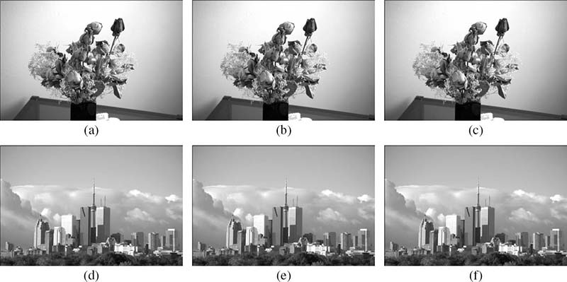
FIGURE 6.11 (See color insert.)
Joint white balancing and color enhancement using the spectral modeling approach: (a,d) ρ = −0.5, (b,e) ρ = 0, and (c,f) ρ = 0.5.

As suggested in the above discussion, various color modeling concepts can be employed within the presented framework. For example, in addition to the color ratio-based calculations, the reference vector ${\hat{x}}_{(r, s)}$ can be obtained as ${\hat{x}}_{(r, s) k} = x_{(r, s) 2} + {\bar{x}}_{k} - {\bar{x}}_{2}$ and ${\hat{x}}_{(r, s) 2} = x_{(r, s) k} + {\bar{x}}_{2} - {\bar{x}}_{k}$ for α_(r,s)k with k = ∈ {1,3} using the color difference concept presented in Equation 6.19. The enumeration of all available options or the determination of the optimal design configuration according to some criteria is beyond the scope of this chapter.

Images

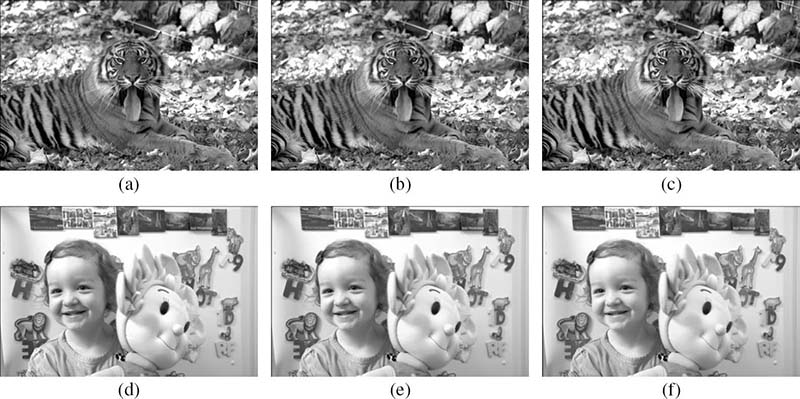
FIGURE 6.12 (See color insert.)
Joint white balancing and color enhancement using the combinatorial approach: (a,d) w = 0.5, (b,e) w = 0, and (c,f) w = −0.5.

6.4.2 Combinatorial Approach

Spectral modeling is not the only available option to combine the global and local reference color vectors in order to obtain pixel-adaptive gains. This combination function can be as simple as a weighting scheme with a tunable parameter assigned to control the contribution of the local gains and its complementary value assigned to control the contribution of the global gains [24], [50]:

$\begin{matrix} α_{(r, s) k} = w \frac{x_{(r, s) 2}}{x_{(r, s) k}} + (1 - w) \frac{{\bar{x}}_{2}}{{\bar{x}}_{k}}, & for k \in {1, 3}, \end{matrix} (6.31)$

where w is a tunable parameter. Substituting α_(r,s)k in Equation 6.25 with the above gain expression leads to the following:

$\begin{matrix} y_{(r, s) k} = w x_{(r, s) 2} + (1 - w) \frac{{\bar{x}}_{2}}{{\bar{x}}_{k}} x_{(r, s) k}, & for k = 1, 2, 3, \end{matrix} (6.32)$

which is another formulation of pixel-adaptive white balancing.

The amount of color adjustment produced in Equation 6.32 consists of the white balancing term $(1 - w) x_{(r, s) k} {\bar{x}}_{2} / {\bar{x}}_{k}$ and another term wx_(r,s)2, which can be seen as a color enhancement term for certain values of w. Namely, for w = 1 no white balancing is performed, as the method produces achromatic pixels by assigning the value of x_(r,s)2 from the input image to all three components of the output color vector y_{(r, s)}. Reducing the value of w toward zero enhances the amount of coloration from achromatic colors to those generated by white balancing. Further decreasing w, that is, setting w to negative values results in color enhancement, with saturated colors produced for too low values of w. This behavior is demonstrated in Figure 6.12.

Images

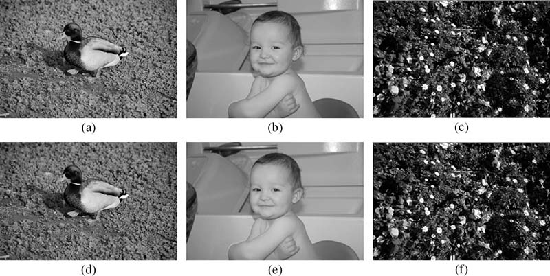
FIGURE 6.13 (See color insert.)
Color enhancement of images with inaccurate white balancing: (a–c) input images and (d–f) their enhanced versions.

6.4.3 Experimental Results

Following the common practice, the presented framework keeps the green channel unchanged using α_(r,s)2 = 1. Color adjustment effects are thus produced through the red and blue channel gains α_{(r, s)1} and α_{(r, s)3}, which are updated in each pixel location of the captured image; that is, for r = 1,2,…, K₁ and s = 1, 2,…, K₂.

The uncorrected color images, such as those shown in Figure 6.9, were produced by demosaicking the scaled raw single-sensor data captured using the Nikon D50 camera with a native resolution of 2014 × 3039 pixels. In order to do the best possible adjustment for the scene illuminant, the global reference vector $x ¯$ was calculated using the pixels in white regions whenever possible.

Figures 6.10 to 6.12 show the results of joint white balancing and color enhancement for some example solutions. As it can be seen, these solutions produce a wide range of color enhancement. Moreover, as demonstrated in Figures 6.11 and 6.12, the color enhancement effects can range from image appearances with suppressed coloration to appearances with rich and vivid colors. The desired amount of color enhancement, according to some criteria, can be easily obtained through parameter tuning.

The next experiment focuses on the effect of color enhancement in situations with inaccurate white-balancing parameters. Figure 6.13 shows both the images with simulated (and perhaps exaggerated) color casts due to incorrect white balancing and the corresponding images after color enhancement. As expected, the color cast is more visible in the images with enhanced colors. In general, any color imperfection, regardless whether it is global (such as color casts) or local (such as color noise) in its nature, gets amplified by the color enhancement process. This behavior is typical also for other color enhancement operations in the camera processing pipeline, including color correction and image rendering (gamma correction, tone curve-based adjustment).

Images

FIGURE 6.14 (See color insert.)
Color adjustment of the final camera images: (a,d) suppressed coloration, (b,e) original coloration, and (c,f) enhanced coloration.

Images

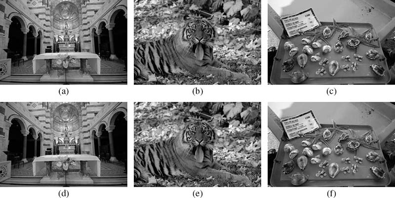
FIGURE 6.15 (See color insert.)
Color enhancement of the final camera images: (a–c) output camera images and (d–f) their enhanced versions.

Finally, Figures 6.14 and 6.15 show the results when the presented framework operates on the final processed camera images. To adapt to such a scenario, one can reasonably assume that the images are already white balanced; this implies that the components of the global reference vector $x ¯$ should be set to the same value. Also in this case, the framework allows for a wide range of color enhancement, which suggests that the visually pleasing images with enhanced colors and improved color contrast can be always found through parameter tuning.

6.4.4 Computational Complexity Analysis

Apart from the actual performance, the computational efficiency is another realistic measure of practicality and usefulness of any algorithm. Several example solutions designed within the presented framework are analyzed below in terms of normalized operations, such as additions (ADDs), subtractions (SUBs), multiplications (MULTs), divisions (DIVS), and comparisons (COMPs).

For the color image with K₁ rows and K₂ columns, the solution defined in Equations 6.25 and 6.26 requires 2K₁K₂ + 2 MULTs and 2K₁K₂ + 2 DIVs to calculate the pixel-adaptive gains, and 2K₁K₂ MULTs to apply these gains to the image. Implementing Equations 6.28 and 6.29 requires 4K₁K₂ + 4 ADDs, 2K₁K₂ + 2 MULTs, and 2K₁K₂ + 2 DIVs to calculate the pixel-adaptive gains and additional 2K₁ K₂ SUBs and 2K₁ K₂ MULTs to apply these gains to the image. The tunable adjustment in Equation 6.30, implemented as a lookup table, will slightly add to the overall complexity. In the case of Equation 6.32, the adjustment process requires 2K₁K₂ ADDs, 1 SUB, 4K₁K₂ + 2 MULTs, and 2 DIVs. In addition to the above numbers, 3K₁K₂ − 3 ADDs and 3 DIVs are needed when the global reference vector $x ¯$ in Equation 6.24 is calculated using all the pixels, or 3|ζ| − 3 ADDs, 3 DIVs, and 3K₁K₂ COMPs when $x ¯$ is calculated using the selected pixels. As can be seen, all the example solutions have a very reasonable computational complexity, which should allow their efficient implementation in various real-time imaging applications.

Moreover, as reported in Reference [25], the execution of various solutions designed within the presented framework on a laptop equipped with an Intel Pentium IV 2.40 GHz processor, 512 MB RAM box, Windows XP operating system, and MS Visual C++ 5.0 programming environment can take (on average) between 0.4 and 0.85 seconds to process a 2014 × 3039 color image. Additional performance improvements are expected through extensive software optimization. Both the computational complexity analysis and the reported execution time suggest that the presented framework is cost-effective.

Finally, it should be noted that this chapter focuses on the color manipulation operations performed on full-color data. In the devices that acquire images using the image sensor covered by the color filter array, the full-color image is obtained using the process known as demosaicking or color interpolation. However, as discussed in References [24], [25], and [50], the presented framework is flexible and can be applied before or even combined with the demosaicking step. Thus, additional computational savings can be achieved.

6.4.5 Discussion

Numerous solutions can be designed within the presented framework by applying the underlying principle of mixing the global and local spectral characteristics of the captured image. In addition to using the actual pixel to produce the color enhancement effect, the framework allows extracting the local image characteristics using the samples inside a local neighborhood of the pixel being adjusted. These neighborhoods can be determined by dividing the entire image either into non-overlapping or overlapping blocks, and then selecting a block that, for example, contains the pixel location or minimizes the distance between its center and the pixel location being adjusted. However, such block-based processing may significantly increase the computational complexity compared to true pixel-adaptive methods, such as the example solutions presented in this chapter.

The presented framework can operate in conjunction with the white balancing gains recorded by the camera. This can be done through the replacement of ratios ${\bar{x}}_{2} / {\bar{x}}_{k}$ , for k ∈ {1,3}, with the actual gains indicated by the camera for each of the respective color channels. If the gain associated with the green channel is not equal to one, then the white balancing gains should be normalized by the gain value associated with the green channel prior to performing the replacement.

In summary, the presented framework, which integrates white balancing and pixeladaptive color enhancement operations, can be readily used in numerous digital camera and color imaging applications. The example solutions designed within this framework are flexible; they can be used in conjunction with various existing white balancing techniques and allow for both global or localized control of the color enhancement process. The framework is computationally efficient, has an excellent performance, and can produce visually pleasing color images with enhanced coloration and improved color contrast. The framework can be seen as an effective solution that complements traditional color correction, color saturation, and tone curve adjustment operations in the digital imaging pipeline or a stand-alone color enhancement tool suitable for image editing software and online image processing applications.

6.5 Color Image Quality Evaluation

The performance of color image processing methods, in terms of image quality, is usually evaluated using the subjective evaluation approach and the objective evaluation approach.

6.5.1 Subjective Assessment

Since most of the images are typically intended for human inspection, the human opinion on visual quality is very important [51]. Statistically meaningful results are usually obtained by conducting a large-scale study where human observers view and rate images, presented either in specific or random order and under identical viewing conditions, using a predetermined rating scale [52]. For example, considering the scope of this chapter, the score can range from one to five, reflecting poor, fair, good, very good, and excellent white balancing, respectively. Using the same score scale, the presence of any distortion, such as color artifacts and posterization effects, introduced to the image through the color adjustment process can be evaluated as very disruptive, disruptive, destructive but not disruptive, perceivable but not destructive, and imperceivable.

6.5.2 Objective Assessment

In addition to subjective assessment of image quality, automatic assessment of visual quality should be performed whenever possible, preferably using the methods that are capable of assessing the perceptual quality of images or can produce the scores that correlate well with subjective opinion.

In the CIE-Luv or CIE-Lab color space, perceptual differences between two colors can be measured using the Euclidean distance. This approach is frequently used in various simulations to evaluate the difference between the original image and its processed version. It is also common that the image quality is evaluated with respect to the known ground-truth data of some object(s) present in the scene, typically a target, such as the Macbeth color checker shown in Figure 6.1.

If the image is in the RGB format, the procedure includes the conversion of each pixel from the RGB values to the corresponding XYZ values using Equation 6.4, and then from these XYZ values to the target Luv or Lab values using the conversion formulas described in Section 6.2.2.2. Operating on the pixel level, the resulting perceptual difference between the two color vectors can be expressed as follows [29]:

$Δ E_{u v}^{*} = \sqrt{{(L_{1}^{*} - L_{2}^{*})}^{2} + {(u_{1}^{*} - u_{2}^{*})}^{2} + {(v_{1}^{*} - v_{2}^{*})}^{2}}, (6.33)$

$Δ E_{b}^{*} = \sqrt{{(L_{1}^{*} - L_{2}^{*})}^{2} + {(a_{1}^{*} - a_{2}^{*})}^{2} + {(b_{1}^{*} - b_{2}^{*})}^{2}} . (6.34)$

The perceptual difference between the two images is usually calculated as an average of ΔE errors obtained in each pixel location. Psychovisual experiments have shown that the value of ΔE equal to unity represents a just noticeable difference (JND) in either of these two color models [53], although higher JND values may be needed to account for the complexity of visual information in pictorial scenes.

Since any color can be described in terms of its lightness, chroma, and hue, the CIE-Lab error can be equivalently expressed as follows [29], [33]:

$Δ E_{a b}^{*} = \sqrt{{(Δ L_{a b}^{*})}^{2} + {(Δ C_{a b}^{*})}^{2} + {(Δ H_{a b}^{*})}^{2}}, (6.35)$

where $Δ L_{a b}^{*} = L_{1}^{*} - L_{2}^{*}$ denotes the difference in lightness,

$Δ C_{a b}^{*} = C_{1}^{*} - C_{2}^{*} = \sqrt{{(a_{1}^{*})}^{2} + {(b_{1}^{*})}^{2}} - \sqrt{{(a_{2}^{*})}^{2} + {(b_{2}^{*})}^{2}} (6.36)$

denotes the difference in chroma, and

$Δ H_{a b}^{*} = \sqrt{{(a_{1}^{*} - a_{2}^{*})}^{2} + {(b_{1}^{*} - b_{2}^{*})}^{2} - {(Δ C_{a b}^{*})}^{2}} (6.37)$

denotes a measure of hue difference. Note that the hue angle can be expressed as $h_{a b}^{*} =$ arctan(b/a).

A more recent ΔE formulation weights the chroma and hue components by a function of chroma [54]:

$Δ E_{94}^{*} = \sqrt{{(\frac{Δ L_{a b}^{*}}{k_{L} S_{L}})}^{2} + {(\frac{Δ C_{a b}^{*}}{k_{C} S_{C}})}^{2} + {(\frac{Δ H_{a b}^{*}}{k_{H} S_{H}})}^{2}}, (6.38)$

where S_L = 1, $S_{H} = 1 + 0.015 \sqrt{C_{1}^{*} C_{2}^{*}}$ , $S_{C} = 1 + 0.045 \sqrt{C_{1}^{*} C_{2}^{*}}$ , and k_L = k_H = k_C = 1 for reference conditions. More sophisticated formulations of the ΔE measure can be found in References [55], [56], and [57], which employs spatial filtering to obtain an improved measure for pictorial scenes.

6.6 Conclusion

This chapter presented a framework that can simultaneously perform white balancing and color enhancement. This framework takes advantage of pixel-adaptive processing, which combines the local and global spectral characteristics of the captured visual data in order to produce the output image with the desired color appearance. Various specific solutions were presented as example methods based on relatively simple but yet powerful spectral modeling or combinatorial principles.

The framework is flexible, as it permits a wide range of functions that can follow the underlying concept of adaptive white balancing using a localized reference color vector that blends the spectral characteristics of the estimated illumination and the actual pixel. An additional degree of freedom in the design can be achieved through various tunable parameters that may be associated with such functions. The variety of such functions and efficient design methodology makes the presented framework very valuable in modern digital imaging and multimedia systems that attempt to mimic the human visual perception and use color as a cue for better image understanding and improved processing performance.

Acknowledgment

The framework presented in this chapter was invented during the author’s employment at Epson Canada Ltd. at Toronto, ON, Canada.

References

[1] R. Lukac, Single-Sensor Imaging: Methods and Applications for Digital Cameras. Boca Raton, FL, USA: CRC Press / Taylor & Francis, September 2008.

[2] R. Lukac, Computational Photography: Methods and Applications. Boca Raton, FL, USA: CRC Press / Taylor & Francis, October 2010.

[3] J. Adams, K. Parulski, and K. Spaulding, “Color processing in digital cameras,” IEEE Micro, vol. 18, no. 6, pp. 20–30, November 1998.

[4] R. Lukac and K.N. Plataniotis, “Color filter arrays: Design and performance analysis,” IEEE Transactions on Consumer Electronics, vol. 51, no. 4, pp. 1260–1267, November 2005.

[5] K. Hirakawa and P.J. Wolfe, “Spatio-spectral sampling and color filter array design,” in Single-Sensor Imaging: Methods and Applications for Digital Cameras, R. Lukac (ed.), Boca Raton, FL, USA: CRC Press / Taylor & Francis, September 2008, pp. 137–151.

[6] P.L.P. Dillon, D.M. Lewis, and F.G. Kaspar, “Color imaging system using a single CCD area array,” IEEE Journal of Solid-State Circuits, vol. 13, no. 1, pp. 28–33, February 1978.

[7] B.T. Turko and G.J. Yates, “Low smear CCD camera for high frame rates,” IEEE Transactions on Nuclear Science, vol. 36, no. 1, pp. 165–169, February 1989.

[8] A.J. Blanksby and M.J. Loinaz, “Performance analysis of a color CMOS photogate image sensor,” IEEE Transactions on Electron Devices, vol. 47, no. 1, pp. 55–64, January 2000.

[9] D. Doswald, J. Haflinger, P. Blessing, N. Felber, P. Niederer, and W. Fichtner, “A 30-frames/s megapixel real-time CMOS image processor,” IEEE Journal of Solid-State Circuits, vol. 35, no. 11, pp. 1732–1743, November 2000.

[10] K. Parulski and K.E. Spaulding, “Color image processing for digital cameras,” in Digital Color Imaging Handbook, G. Sharma (ed.), Boca Raton, FL, USA: CRC Press, December 2002, pp. 728–757.

[11] R. Lukac, “Single-sensor digital color imaging fundamentals,” in Single-Sensor Imaging: Methods and Applications for Digital Cameras, R. Lukac (ed.), Boca Raton, FL, USA: CRC Press / Taylor & Francis, September 2008, pp. 1–29.

[12] J.E. Adams and J.F. Hamilton, “Digital camera image processing chain design,” in Single-Sensor Imaging: Methods and Applications for Digital Cameras, R. Lukac (ed.), Boca Raton, FL, USA: CRC Press / Taylor & Francis, September 2008, pp. 67–103.

[13] K. Barnard, L. Martin, A. Coath, and B. Funt, “A comparison of computational color constancy algorithms – Part I: Experiments with image data,” IEEE Transactions on Image Processing vol. 11, no. 9, pp. 985–996, September 2002.

[14] G.D. Finlayson, “Three-, two-, one-, and six-dimensional color constancy,” in Color Image Processing: Methods and Applications, R. Lukac and K.N. Plataniotis (eds.), Boca Raton, FL, USA: CRC Press / Taylor & Francis, October 2006, pp. 55–74.

[15] J. Lee, Y. Jung, B. Kim, and S. Ko, “An advanced video camera system with robust AF, AE, and AWB control,” IEEE Transactions on Consumer Electronics, vol. 47, no. 3, pp. 694–699, August 2001.

[16] G. Sharma, “Color fundamentals for digital imaging,” in Digital Color Imaging Handbook, G. Sharma (ed.), Boca Raton, FL, USA: CRC Press / Taylor & Francis, December 2002, pp. 1–113.

[17] E. Reinhard, E.A. Khan, A.O. Akyuz, and G.M. Johnson, Color Imaging: Fundamentals and Applications. Wellesley, MA, USA: AK Peters, July 2008.

[18] G.M. Johnson and M.D. Fairchild, “Visual psychophysics and color appearance,” in Digital Color Imaging Handbook, G. Sharma (ed.), Boca Raton, FL, USA: CRC Press / Taylor & Francis, December 2002, pp. 173–238.

[19] “Lighting design glossary,” in Lighting Design and Simulation Knowledgebase, Available online, http://www.schorsch.com/en/kbase/glossary/adaptation.html.

[20] E. Lam and G.S.K. Fung, “Automatic white balancing in digital photography,” in Single-Sensor Imaging: Methods and Applications for Digital Cameras, LukacR. (ed.), Boca Raton, FL, USA: CRC Press / Taylor & Francis, September 2008, pp. 267–294.

[21] N. Sampat, S. Venkataraman, and R. Kremens, “System implications of implementing white balance on consumer digital cameras,” Proceedings of SPIE, vol. 3965, pp. 362–368, January 2000.

[22] C.C. Weng, H. Chen, and C.S. Fuh, “A novel automatic white balance method for digital still cameras,” in Proceedings of the IEEE International Symposium on Circuits and Systems, Kobe, Japan, May 2005, vol. 4, pp. 3801–3804.

[23] N. Kehtarnavaz, N. Kim, and M. Gamadia, “Real-time auto white balancing for digital cameras using discrete wavelet transform-based scoring,” Journal of Real-Time Image Processing, vol. 1, no. 1, pp. 89–97, October 2006.

[24] R. Lukac, “Automatic white balancing of a digital image,” U.S. Patent7 889 245, February 2011.

[25] R. Lukac, “New framework for automatic white balancing of digital camera images,” Signal Processing, vol. 88, no. 3, pp. 582–593, March 2008.

[26] R. Gonzalez and R.E. Woods, Digital Image Processing. Reading, MA, USA: Prentice Hall, 3rd edition, August 2007.

[27] E. Giorgianni and T. Madden, Digital Color Management. Reading, MA, USA: Addison-Wesley, 2nd edition, January 2009.

[28] G. Wyszecki and W.S. Stiles, Color Science: Concepts and Methods, Quantitative Data and Formulas. New York, USA: Wiley-Interscience, 2nd edition, August 2000.

[29] H.J. Trussell, E. Saber, and M. Vrhel, “Color image processing,” IEEE Signal Processing Magazine, vol. 22, no. 1, pp. 14–22, January 2005.

[30] M. Stokes, M. Anderson, S. Chandrasekar, and R. Motta, “A standard default color space for the internet – sRGB,” Technical report, Available online, http://www.w3.org/Graphics/Color/sRGB.html.

[31] R.W.G. Hunt, Measuring Colour. Chichester, UK: Wiley, 4th edition, December 2011.

[32] S. Susstrunk, R. Buckley, and S. Swen, “Standard RGB color spaces,” in Proceedings of the Seventh Color Imaging Conference: Color Science, Systems, and Applications, Scottsdale, AZ, USA, November 1999, pp. 127–134.

[33] S. Susstrunk, “Colorimetry,” in Focal Encyclopedia of Photography, M.R. Peres (ed.), Burlington, MA, USA: Focal Press / Elsevier, 4th edition, 2007, pp. 388–393.

[34] R.G. Kuehni, Color Space and Its Divisions: Color Order from Antiquity to the Present. Hoboken, NJ, USA: Wiley-Interscience, March 2003.

[35] C.A. Poynton, A Technical Introduction to Digital Video. Toronto, ON, Canada: Prentice Hall, January 1996.

[36] A. Sharma, “ICC color management: Architecture and implementation,” in Color Image Processing: Methods and Applications, R. Lukac and K.N. Plataniotis (eds.), Boca Raton, FL, USA: CRC Press / Taylor & Francis, October 2006, pp. 1–27.

[37] R. Lukac, B. Smolka, K. Martin, K.N. Plataniotis, and A.N. Venetsanopulos, “Vector filtering for color imaging,” IEEE Signal Processing Magazine, vol. 22, no. 1, pp. 74–86, January 2005.

[38] J. Gomes and L. Velho, Image Processing for Computer Graphics. New York, USA: Springer-Verlag, May 1997.

[39] R. Lukac and K.N. Plataniotis, “Single-sensor camera image processing,” in Color Image Processing: Methods and Applications, R. Lukac and K.N. Plataniotis (eds.), Boca Raton, FL, USA: CRC Press / Taylor & Francis, October 2006, pp. 363–392.

[40] R. Lukac and K.N. Plataniotis, “Normalized color-ratio modeling for CFA interpolation,” IEEE Transactions on Consumer Electronics, vol. 50, no. 2, pp. 737–745, May 2004.

[41] D.R. Cok, “Signal processing method and apparatus for producing interpolated chrominance values in a sampled color image signal.” U.S. Patent4 642 678, February 1987.

[42] J. Adams, “Design of practical color filter array interpolation algorithms for digital cameras,” Proceedings of SPIE, vol. 3028, pp. 117–125, February 1997.

[43] G.D. Finlayson, S.D. Hordley, and P.M. Hubel, “Color by correlation: A simple, unifying framework for color constancy,” IEEE Transactions on Pattern Analysis and Machine Intelligence, vol. 23, no. 11, pp. 1209–1221, November 2001.

[44] N. Kehtarnavaz, H. Oh, and Y. Yoo, “Development and real-time implementation of auto white balancing scoring algorithm,” Real-Time Imaging, vol. 8, no. 5, pp. 379–386, October 2002.

[45] E.Y. Lam, “Combining gray world and Retinex theory for automatic white balance in digital photography,” in Proceedings of the International Symposium on Consumer Electronics, Macau, China, June 2005, pp. 134–139.

[46] J. Huo, Y. Chang, J. Wang, and X. Wei, “Robust automatic white balance algorithm using gray color points in images,” IEEE Transactions on Consumer Electronics, vol. 52, no. 2, pp. 541–546, May 2006.

[47] G. Sapiro, “Color and illuminant voting,” IEEE Transactions on Pattern Analysis and Machine Intelligence, vol. 21, no. 11, pp. 1210–1215, November 1999.

[48] S. Bianco, F. Gasparini, and R. Schettini, “Combining strategies for white balance,” Proceedings of SPIE, vol. 6502, id. 65020D, January 2007.

[49] R. Lukac, “Refined automatic white balancing,” IET Electronics Letters, vol. 43, no. 8, pp. 445–446, April 2007.

[50] R. Lukac, “Joint automatic demosaicking and white balancing,” U.S. Patent8 035 698, October 2011.

[51] A.K. Moorthy, K. Seshadrinathan, and A.C. Bovik, “Image and video quality assessment: Perception, psychophysical models, and algorithms,” in Perceptual Imaging: Methods and Applications, R. Lukac (ed.), Boca Raton, FL, USA: CRC Press / Taylor & Francis, 2012.

[52] K.N. Plataniotis and A.N. Venetsanopoulos, Color Image Processing and Applications. New York, USA: Springer-Verlag, 2nd edition, December 2010.

[53] D.F. Rogers and R.E. Earnshaw, Computer Graphics Techniques: Theory and Practice. New York, USA: Springer-Verlag, October 2001.

[54] CIE publication No 116, Industrial colour difference evaluation. Central Bureau of the CIE, 1995

[55] M.R. Luo, G. Cui, and B. Rigg, “The development of the CIE 2000 colour difference formula: CIEDE2000,” Color Research and Applications, vol. 26, no. 5, pp. 340–350, October 2001.

[56] M.R. Luo, G. Cui, B. Rigg, “Further comments on CIEDE2000,” Color Research and Applications, vol. 27, no. 2, pp. 127–128, April 2002.

[57] B. Wandell, “S-CIELAB: A spatial extension of the CIE L*a*b* DeltaE color difference metric.” Available online, http://white.stanford.edu/~brian/scielab/.

..................Content has been hidden....................

You can't read the all page of ebook, please click here login for view all page.

Table of Contents for 6 Joint White Balancing and Color Enhancement

Create new playlist

Sign In

Sign Up

Table of Contents for
6 Joint White Balancing and Color Enhancement