Tree models are ubiquitous in machine learning. They are naturally suited to divide and conquer iterative algorithms. One of the main advantages of decision tree models is that they are naturally easy to visualize and conceptualize. They allow inspection and do not just give an answer. For example, if we have to predict a category, we can also expose the logical steps that give rise to a particular result. Also tree models generally require less data preparation than other models and can handle numerical and categorical data. On the down side, tree models can create overly complex models that do not generalize to new data very well. Another potential problem with tree models is that they can become very sensitive to changes in the input data and, as we will see later, this problem can be mitigated against using them as ensemble learners.

An important difference between decision trees and the hypothesis mapping used in the previous section is that the tree model does not use internal disjunction on features with more than two values but instead branches on each value. We can see this with the size feature in the following diagram:

Another point to note is that decision trees are more expressive than the conjunctive hypothesis and we can see this here, where we have been able to separate the data where the conjunctive hypothesis covered negative examples. This expressiveness, of course, comes with a price: the tendency to overfit on training data. A way to force generalization and reduce overfitting is to introduce an inductive bias toward less complex hypotheses.

We can quite easily implement our little example using the Sklearn DecisionTreeClassifier and create an image of the resultant tree:

from sklearn import tree

names=['size','scale','fruit','butt']
labels=[1,1,1,1,1,0,0,0]

p1=[2,1,0,1]
p2=[1,1,0,1]
p3=[1,1,0,0]
p4=[1,1,0,0]
n1=[0,0,0,0]
n2=[1,0,0,0]
n3=[0,0,1,0]
n4=[1,1,0,0]
data=[p1,p2,p3,p4,n1,n2,n3,n4]

def pred(test, data=data):
    dtre=tree.DecisionTreeClassifier()
    dtre=dtre.fit(data,labels)
    print(dtre.predict([test]))
    with open('data/treeDemo.dot', 'w') as f:
        f=tree.export_graphviz(dtre,out_file=f,
                               feature_names=names)
pred([1,1,0,1])

Running the preceding code creates a treeDemo.dot file. The decision tree classifier, saved as a .dot file, can be converted into an image file such as a .png, .jpeg or .gif using the Graphiz graph visualization software. You can download Graphviz from http://graphviz.org/Download.php. Once you have it installed, use it to convert the .dot file into an image file format of your choice.

This gives you a clear picture of how the decision tree has been split.

We can see from the full tree that we recursively split on each node, increasing the proportion of samples of the same class with each split. We continue down nodes until we reach a leaf node where we aim to have a homogeneous set of instances. This notion of purity is an important one because it determines how each node is split and it is behind the Gini values in the preceding diagram.

Purity

How do we understand the usefulness of each feature in relation to being able to split samples into classes that contain minimal or no samples from other classes? What are the indicative sets of features that give a class its label? To answer this, we need to consider the idea of purity of a split. For example, consider we have a set of Boolean instances, where D is split into D1 and D2. If we further restrict ourselves to just two classes, D^pos and D^neg, we can see that the optimum situation is where D is split perfectly into positive and negative examples. There are two possibilities for this: either where D1^pos = D^pos and D1^neg = {}, or D1^neg = D^neg and D1^pos = {}.

If this is true, then the children of the split are said to be pure. We can measure the impurity of a split by the relative magnitude of n^pos and n^neg. This is the empirical probability of a positive class and it can be defined by the proportion p=n^pos /(n^pos + n^neg). There are several requirements for an impurity function. First, if we switch the positive and negative class (that is, replace p with 1-p) then the impurity should not change. Also the function should be zero when p=0 or p=1, and it should reach its maximum when p=0.5. In order to split each node in a meaningful way, we need an optimization function with these characteristics.

There are three functions that are typically used for impurity measures, or splitting criteria, with the following properties.

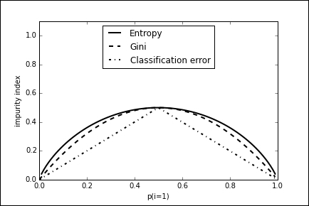
• Minority class: This is simply a measure of the proportion of misclassified examples assuming we label each leaf with the majority class. The higher this proportion is, the greater the number of errors and the greater the impurity of the split. This is sometimes called the classification error, and is calculated as min(p,1-p).
• Gini index: This is the expected error if we label examples either positive, with probability p, or negative, with probability 1-p. Sometimes, the square root of the Gini index is used as well, and this can have some advantages when dealing with highly skewed data where a large proportion of samples belongs to one class.
• Entropy: This measure of impurity is based on the expected information content of the split. Consider a message telling you about the class of a series of randomly drawn samples. The purer the set of samples, the more predictable this message becomes, and therefore the smaller the expected information. Entropy is measured by the following formula:

These three splitting criteria, for a probability range of between 0 and 1, are plotted in the following diagram. The entropy criteria are scaled by 0.5 to enable them to be compared to the other two. We can use the output from the decision tree to see where each node lies on this curve.