
Implementations of artificial neural networks can be quite complex, and it is always a good idea to manually check that we have implemented backpropagation correctly. In this section, we will talk about a simple procedure called gradient checking, which is essentially a comparison between our analytical gradients in the network and numerical gradients. Gradient checking is not specific to feedforward neural networks but can be applied to any other neural network architecture that uses gradient-based optimization. Even if you are planning to implement more trivial algorithms using gradient-based optimization, such as linear regression, logistic regression, and support vector machines, it is generally not a bad idea to check if the gradients are computed correctly.
In the previous sections, we defined a cost function ![]() where
where ![]() is the matrix of the weight coefficients of an artificial network. Note that
is the matrix of the weight coefficients of an artificial network. Note that ![]() is—roughly speaking—a "stacked" matrix consisting of the matrices
is—roughly speaking—a "stacked" matrix consisting of the matrices ![]() and
and ![]() in a multi-layer perceptron with one hidden unit. We defined
in a multi-layer perceptron with one hidden unit. We defined ![]() as the
as the ![]() -dimensional matrix that connects the input layer to the hidden layer, where
-dimensional matrix that connects the input layer to the hidden layer, where ![]() is the number of hidden units and
is the number of hidden units and ![]() is the number of features (input units). The matrix
is the number of features (input units). The matrix ![]() that connects the hidden layer to the output layer has the dimensions
that connects the hidden layer to the output layer has the dimensions ![]() , where
, where ![]() is the number of output units. We then calculated the derivative of the cost function for a weight
is the number of output units. We then calculated the derivative of the cost function for a weight ![]() as follows:
as follows:

Remember that we are updating the weights by taking an opposite step towards the direction of the gradient. In gradient checking, we compare this analytical solution to a numerically approximated gradient:

Here, ![]() is typically a very small number, for example 1e-5 (note that 1e-5 is just a more convenient notation for 0.00001). Intuitively, we can think of this finite difference approximation as the slope of the secant line connecting the points of the cost function for the two weights
is typically a very small number, for example 1e-5 (note that 1e-5 is just a more convenient notation for 0.00001). Intuitively, we can think of this finite difference approximation as the slope of the secant line connecting the points of the cost function for the two weights ![]() and
and ![]() (both are scalar values), as shown in the following figure. We are omitting the superscripts and subscripts for simplicity.
(both are scalar values), as shown in the following figure. We are omitting the superscripts and subscripts for simplicity.

An even better approach that yields a more accurate approximation of the gradient is to compute the symmetric (or centered) difference quotient given by the two-point formula:

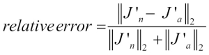
Typically, the approximated difference between the numerical gradient ![]() and analytical gradient
and analytical gradient ![]() is then calculated as the L2 vector norm. For practical reasons, we unroll the computed gradient matrices into flat vectors so that we can calculate the error (the difference between the gradient vectors) more conveniently:
is then calculated as the L2 vector norm. For practical reasons, we unroll the computed gradient matrices into flat vectors so that we can calculate the error (the difference between the gradient vectors) more conveniently:
One problem is that the error is not scale invariant (small errors are more significant if the weight vector norms are small too). Thus, it is recommended to calculate a normalized difference:
Now, we want the relative error between the numerical gradient and the analytical gradient to be as small as possible. Before we implement gradient checking, we need to discuss one more detail: what is the acceptable error threshold to pass the gradient check? The relative error threshold for passing the gradient check depends on the complexity of the network architecture. As a rule of thumb, the more hidden layers we add, the larger the difference between the numerical and analytical gradient can become if backpropagation is implemented correctly. Since we have implemented a relatively simple neural network architecture in this chapter, we want to be rather strict about the threshold and define the following rules:
- Relative error <= 1e-7 means everything is okay!
- Relative error <= 1e-4 means the condition is problematic, and we should look into it.
- Relative error > 1e-4 means there is probably something wrong in our code.
Now we have established these ground rules, let's implement gradient checking. To do so, we can simply take the NeuralNetMLP class that we implemented previously and add the following method to the class body:
def _gradient_checking(self, X, y_enc, w1,
                       w2, epsilon, grad1, grad2):
    """ Apply gradient checking (for debugging only)

    Returns
    ---------
    relative_error : float
      Relative error between the numerically
      approximated gradients and the backpropagated gradients.

    """
    num_grad1 = np.zeros(np.shape(w1))
    epsilon_ary1 = np.zeros(np.shape(w1))
    for i in range(w1.shape[0]):
        for j in range(w1.shape[1]):
            epsilon_ary1[i, j] = epsilon
            a1, z2, a2, z3, a3 = self._feedforward(
                                           X,
                                           w1 - epsilon_ary1,
                                           w2)
            cost1 = self._get_cost(y_enc,
                                   a3,
                                   w1-epsilon_ary1,
                                   w2)
            a1, z2, a2, z3, a3 = self._feedforward(
                                         X,
                                         w1 + epsilon_ary1,
                                         w2)
            cost2 = self._get_cost(y_enc,
                                   a3,
                                   w1 + epsilon_ary1,
                                   w2)
            num_grad1[i, j] = (cost2 - cost1) / (2 * epsilon)
            epsilon_ary1[i, j] = 0

    num_grad2 = np.zeros(np.shape(w2))
    epsilon_ary2 = np.zeros(np.shape(w2))
    for i in range(w2.shape[0]):
        for j in range(w2.shape[1]):
            epsilon_ary2[i, j] = epsilon
            a1, z2, a2, z3, a3 = self._feedforward(
                                            X,
                                            w1,
                                            w2 - epsilon_ary2)
            cost1 = self._get_cost(y_enc,
                                   a3,
                                   w1,
                                   w2 - epsilon_ary2)
            a1, z2, a2, z3, a3 = self._feedforward(
                                          X,
                                          w1,
                                          w2 + epsilon_ary2)
            cost2 = self._get_cost(y_enc,
                                   a3,
                                   w1,
                                   w2 + epsilon_ary2)
            num_grad2[i, j] = (cost2 - cost1) / (2 * epsilon)
            epsilon_ary2[i, j] = 0

    num_grad = np.hstack((num_grad1.flatten(),
                          num_grad2.flatten()))
    grad = np.hstack((grad1.flatten(), grad2.flatten()))
    norm1 = np.linalg.norm(num_grad - grad)
    norm2 = np.linalg.norm(num_grad)
    norm3 = np.linalg.norm(grad)
    relative_error = norm1 / (norm2 + norm3)
    return relative_error
The _gradient_checking code seems rather simple. However, my personal recommendation is to keep it as simple as possible. Our goal is to double-check the gradient computation, so we want to make sure that we do not introduce any additional mistakes in gradient checking by writing efficient but complex code. Next, we only need to make a small modification to the fit method. In the following code, I omitted the code at the beginning of the fit function for clarity, and the only lines that we need to add to the method are implemented between the comments ## start gradient checking and ## end gradient checking:
class MLPGradientCheck(object):
    [...]
    def fit(self, X, y, print_progress=False):
        [...]
                # compute gradient via backpropagation
                grad1, grad2 = self._get_gradient(
                                       a1=a1,
                                       a2=a2,
                                       a3=a3,
                                       z2=z2,
                                       y_enc=y_enc[:, idx],
                                       w1=self.w1,
                                       w2=self.w2)

                ## start gradient checking

                grad_diff = self._gradient_checking(
                                     X=X[idx],
                                     y_enc=y_enc[:, idx],
                                     w1=self.w1,
                                     w2=self.w2,
                                     epsilon=1e-5,
                                     grad1=grad1,
                                     grad2=grad2)
                if grad_diff <= 1e-7:
                    print('Ok: %s' % grad_diff)
                elif grad_diff <= 1e-4:
                    print('Warning: %s' % grad_diff)
                else:
                    print('PROBLEM: %s' % grad_diff)

                ## end gradient checking

                # update weights; [alpha * delta_w_prev]
                # for momentum learning
                delta_w1 = self.eta * grad1
                delta_w2 = self.eta * grad2
                self.w1 -= (delta_w1 +
                           (self.alpha * delta_w1_prev))
                self.w2 -= (delta_w2 +
                           (self.alpha * delta_w2_prev))
                delta_w1_prev = delta_w1
                delta_w2_prev = delta_w2

        return self
Assuming that we named our modified multi-layer perceptron class MLPGradientCheck, we can now initialize a new MLP with 10 hidden layers. Also, we disable regularization, adaptive learning, and momentum learning. In addition, we use regular gradient descent by setting minibatches to 1. The code is as follows:
>>> nn_check = MLPGradientCheck(n_output=10,
                                n_features=X_train.shape[1],
                                n_hidden=10,
                                l2=0.0,
                                l1=0.0,
                                epochs=10,
                                eta=0.001,
                                alpha=0.0,
                                decrease_const=0.0,
                                minibatches=1,
                                random_state=1)
One downside of gradient checking is that it is computationally very, very expensive. Training a neural network with gradient checking enabled is so slow that we really only want to use it for debugging purposes. For this reason, it is not uncommon to run gradient checking only on a handful of training samples (here, we choose 5). The code is as follows:
>>> nn_check.fit(X_train[:5], y_train[:5], print_progress=False)
Ok: 2.56712936241e-10
Ok: 2.94603251069e-10
Ok: 2.37615620231e-10
Ok: 2.43469423226e-10
Ok: 3.37872073158e-10
Ok: 3.63466384861e-10
Ok: 2.22472120785e-10
Ok: 2.33163708438e-10
Ok: 3.44653686551e-10
Ok: 2.17161707211e-10
As we can see from the code output, our multi-layer perceptron passes this test with excellent results.