
We should know that there is a hierarchy of types for representing data in Python. At the root are immutable objects such as integers, floats, and Boolean. Built on this, we have sequence types. These are ordered sets of objects indexed by non-negative integers. They are iterative objects that include strings, lists, and tuples. Sequence types have a common set of operations such as returning an element (s[i]) or a slice (s[i:j]), and finding the length (len(s)) or the sum (sum(s)). Finally, we have mapping types. These are collections of objects indexed by another collection of key objects. Mapping objects are unordered and are indexed by numbers, strings, or other objects. The built-in Python mapping type is the dictionary.
NumPy builds on these data objects by providing two further objects: an N-dimensional array object (ndarray) and a universal function object (ufunc). The ufunc object provides element-by-element operations on ndarray objects, allowing typecasting and array broadcasting. Typecasting is the process of changing one data type into another, and broadcasting describes how arrays of different sizes are treated during arithmetic operations. There are sub-packages for linear algebra (linalg), random number generation (random), discrete Fourier transforms (fft), and unit testing (testing).
NumPy uses a dtype object to describe various aspects of the data. This includes types of data such as float, integer, and so on, the number of bytes in the data type (if the data is structured), and also, the names of the fields and the shape of any sub arrays. NumPy has several new data types, including the following:
- 8, 16, 32, and 64 bit
intvalues - 16, 32, and 64 bit float values
- 64 and 128 bit complex types
Ndarraystructured array types
We can convert between types using the np.cast object. This is simply a dictionary that is keyed according to destination cast type, and whose value is the appropriate function to perform the casting. Here we cast an integer to a float32:
f= np.cast['f'] (2)
NumPy arrays can be created in several ways such as converting them from other Python data structures, using the built-in array creation objects such as arange(), ones() and zeros(), or from files such as .csv or .html.
Indexing and slicingNumPy builds on the slicing and indexing techniques used in sequences. You should already be familiar with slicing sequences, such as lists and tuples, in Python using the [i:j:k] syntax, where i is the start index, j is the end, and k is the step. NumPy extends this concept of the selection tuple to N-dimensions.
Fire up a Python console and type the following commands:
import numpy as np
a=np.arange(60).reshape(3,4,5)
print(a)
You will observe the following:

This will print the preceding 3 by 4 by 5 array. You should know that we can access each item in the array using a notation such as a[2,3,4]. This returns 59. Remember that indexing begins at 0.
We can use the slicing technique to return a slice of the array.
The following image shows the A[1:2:] array:

Using the ellipse (…), we can select any remaining unspecified dimensions. For example, a[...,1] is equivalent to a[:,:,1]:

You can also use negative numbers to count from the end of the axis:
With slicing, we are creating views; the original array remains untouched, and the view retains a reference to the original array. This means that when we create a slice, even though we assign it to a new variable, if we change the original array, these changes are also reflected in the new array. The following figure demonstrates this:

Here, a and b are referring to the same array. When we assign values in a, this is also reflected in b. To copy an array rather than simply make a reference to it, we use the deep copy() function from the copy package in the standard library:
import copy
c=copy.deepcopy(a)
Here, we have created a new independent array, c. Any changes made in array a will not be reflected in array c.
This slicing functionality can also be used with several NumPy classes as an efficient means of constructing arrays. The numpy.mgrid object, for example, creates a meshgrid object, which provides, in certain circumstances, a more convenient alternative to arange(). Its primary purpose is to build a coordinate array for a specified N-dimensional volume. Refer to the following figure as an example:

Sometimes, we will need to manipulate our data structures in other ways. These include:
- concatenating: By using the
np.r_andnp.c_functions, we can concatenate along one or two axes using the slicing constructs. Here is an example:
Here we have used the complex number 5j as the step size, which is interpreted by Python as the number of points, inclusive, to fit between the specified range, which here is -1 to 1.
- newaxis: This object expands the dimensions of an array:

This creates an extra axis in the first dimension. The following creates the new axis in the second dimension:

You can also use a Boolean operator to filter:
a[a<5]
Out[]: array([0, 1, 2, 3, 4])
- Find the sum of a given axis:

Here we have summed using axis 2.
As you would expect, you can perform mathematical operations such as addition, subtraction, multiplication, as well as the trigonometric functions on NumPy arrays. Arithmetic operations on different shaped arrays can be carried out by a process known as broadcasting. When operating on two arrays, NumPy compares their shapes element-wise from the trailing dimension. Two dimensions are compatible if they are the same size, or if one of them is 1. If these conditions are not met, then a ValueError exception is thrown.
This is all done in the background using the ufunc object. This object operates on ndarrays on a element-by-element basis. They are essentially wrappers that provide a consistent interface to scalar functions to allow them to work with NumPy arrays. There are over 60 ufunc objects covering a wide variety of operations and types. The ufunc objects are called automatically when you perform operations such as adding two arrays using the + operator.
Let's look into some additional mathematical features:
- Vectors: We can also create our own vectorized versions of scalar functions using the
np.vectorize()function. It takes a Pythonscalarfunction or method as a parameter and returns a vectorized version of this function:def myfunc(a,b): def myfunc(a,b): if a > b: return a-b else: return a + b vfunc=np.vectorize(myfunc)
We will observe the following output:

- Polynomial functions: The
poly1dclass allows us to deal with polynomial functions in a natural way. It accepts as a parameter an array of coefficients in decreasing powers. For example, the polynomial, 2x2 + 3x + 4, can be entered by the following:
We can see that it prints out the polynomial in a human-readable way. We can perform various operations on the polynomial, such as evaluating at a point:

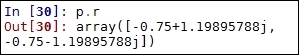
- Find the roots:
We can use asarray(p) to give the coefficients of the polynomial an array so that it can be used in all functions that accept arrays.
As we will see, the packages that are built on NumPy give us a powerful and flexible framework for machine learning.