We mentioned earlier that linear regression can become unstable, that is, highly sensitive to small changes in the training data, if features are correlated. Consider the extreme case where two features are perfectly negatively correlated such that any increase in one feature is accompanied by an equivalent decrease in another feature. When we apply our linear regression algorithm to just these two features, it will result in a function that is constant, so this is not really telling us anything about the data. Alternatively, if the features are positively correlated, small changes in them will be amplified. Regularization helps moderate this.

We saw previously that we could get our hypothesis to more closely fit the training data by adding polynomial terms. As we add these terms, the shape of the function becomes more complicated, and this usually results in the hypothesis overfitting the training data and performing poorly on the test data. As we add features, either directly from the data or the ones we derive ourselves, it becomes more likely that the model will overfit the data. One approach is to discard features that we think are less important. However, we cannot know for certain, in advance, what features may contain relevant information. A better approach is to not discard features but rather to shrink them. Since we do not know how much information each feature contains, regularization reduces the magnitude of all the parameters.

We can simply add the term to the cost function.

The hyper parameter, lambda, controls a tradeoff between two goals—the need to fit the training data, and the need to keep the parameters small to avoid overfitting. We do not apply the regularization parameter to our bias feature, so we separate the update rule for the first feature and add a regularization parameter to all subsequent features. We can write it like this:

Here, we have added our regularization term, λ w_j /m. To see more clearly how this works, we can group all the terms that depend on wj, and our update rule can be rewritten as follows:

The regularization parameter, λ, is usually a small number greater than zero. In order for it to have the desired effect, it is set such that α λ /m is a number slightly less than 1. This will shrink w_j on each iteration of the update.

Now, let's see how we can apply regularization to the normal equation. The equation is as follows:

This is sometimes referred to as the closed form solution. We add the identity matrix, I, multiplied by the regularization parameter. The identity matrix is an (n+1) by (n+1) matrix consisting of ones on the main diagonal and zeros everywhere else.

In some implementations, we might also make the first entry, the top-left corner, of the matrix zero reflect the fact that we are not applying a regularization parameter to the first bias feature. However, in practice, this will rarely make much difference to our model.

When we multiply it with the identity matrix, we get a matrix where the main diagonal contains the value of λ, with all other positions as zero. This makes sure that, even if we have more features than training samples, we will still be able to invert the matrix X^TX. It also makes our model more stable if we have correlated variables. This form of regression is sometimes called ridge regression, and we saw an implementation of this in Chapter 2, Tools and Techniques. An interesting alternative to ridge regression is lasso regression. It replaces the ridge regression regularization term, ∑iwi 2, with ∑i | wi |. That is, instead of using the sum of the squares of the weights, it uses the sum of the average of the weights. The result is that some of the weights are set to 0 and others are shrunk. Lasso regressions tends to be quite sensitive to the regularization parameter. Unlike ridge regression, lasso regression does not have a closed-form solution, so other forms of numerical optimization need to be employed. Ridge regression is sometimes referred to as using the L2 norm, and lasso regularization, the L1 norm.

Finally, we will look at how to apply regularization to logistic regression. As with linear regression, logistic regression can suffer from the same problems of overfitting if our hypothesis functions contain higher-order terms or many features. We can modify our logistic regression cost function to add the regularization parameter, as shown as follows:

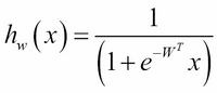
To implement gradient descent for logistic regression, we end up with an equation that, on the surface, looks identical to the one we used for gradient descent for linear regression. However, we must remember that our hypothesis function is the one we used for logistic regression.

Using the hypothesis function, we get the following: