I have already briefly mentioned the idea of thresholding in relation to decision trees, where we transform an ordinal or quantitative feature into a binary feature by finding an appropriate feature value to split on. There are a number of methods, both supervised and unsupervised, that can be used to find an appropriate split in continuous data, for example, using the statistics of central tendency (supervised), such as the mean or median or optimizing an objective function based on criteria such as information gain.

We can go further and create multiple thresholds, transforming a quantitative feature into an ordinal one. Here, we divide a continuous quantitative feature into numerous discrete ordinal values. Each of these values is referred to as a bin, and each bin represents an interval on the original quantitative feature. Many machine learning models require discrete values. It becomes easier and more comprehensible to create rule-based models using discrete values. Discretization also makes features more compact and may make our algorithms more efficient.

One of the most common approaches is to choose bins such that each bin has approximately the same number of instances. This is called equal frequency discretization, and if we apply it to just two bins, then this is the same as using the median as a threshold. This approach can be quite useful because the bin boundaries can be set up in such a way that they represent quantiles. For example, if we have 100 bins, then each bin represents a percentile.

Alternatively, we can choose the boundaries so that each bin has the same interval width. This is called equal width discretization. A way of working out the value of this bin's width interval is simply to divide the feature range by the number of bins. Sometimes, the features do not have an upper or lower limit, and we cannot calculate its range. In this case, integer numbers of standard deviations above and below the mean can be used. Both width and frequency discretization are unsupervised. They do not require any knowledge of the class labels to work.

Let's now turn our attention to supervised discretization. There are essentially two approaches: the top-down or divisive, and the agglomerative or bottom-up approach. As the names suggest, divisive works by initially assuming that all samples belong to the same bin and then progressively splits the bins. Agglomerative methods begin with a bin for each instance and progressively merges these bins. Both methods require some stopping criteria to decide if further splits are necessary.

The process of recursively partitioning feature values through thresholding is an example of divisive discretization. To make this work, we need a scoring function that finds the best threshold for particular feature values. A common way to do this is to calculate the information gain of the split or its entropy. By determining how many positive and negative samples are covered by a particular split, we can progressively split features based on this criterion.

Simple discretization operations can be carried out by the Pandas cut and qcut methods. Consider the following example:

import pandas as pd
import numpy as np
print(pd.cut(np.array([1,2,3,4]), 3, retbins = True, right = False))

Here is the output observed:

Thresholding and discretization, both, remove the scale of a quantitative feature and, depending on the application, this may not be what we want. Alternatively, we may want to add a measure of scale to ordinal or categorical features. In an unsupervised setting, we refer to this as normalization. This is often used to deal with quantitative features that have been measured on a different scale. Feature values that approximate a normal distribution can be converted to z scores. This is simply a signed number of standard deviations above or below the mean. A positive z score indicates a number of standard deviations above the mean, and a negative z score indicates the number of standard deviations below the mean. For some features, it may be more convenient to use the variance rather than the standard deviation.

A stricter form of normalization expresses a feature on a 0 to 1 scale. If we know a features range, we can simply use a linear scaling, that is, divide the difference between the original feature value and the lowest value with the difference between the lowest and highest value. This is expressed in the following:

Here, f_n is the normalized feature, f is the original feature, and l and h are the lowest and highest values, respectively. In many cases, we may have to guess the range. If we know something about a particular distribution, for example, in a normal distribution more than 99% of values are likely to fall within +3 or -3 standard deviations of the mean, then we can write a linear scaling such as the following:

Here, μ is the mean and ơ is the standard deviation.

Sometimes, we need to add scale information to an ordinal or categorical feature. This is called feature calibration. It is a supervised feature transformation that has a number of important applications. For example, it allows models that require scaled features, such as linear classifiers, to handle categorical and ordinal data. It also gives models the flexibility to treat features as ordinal, categorical, or quantitative. For binary classification, we can use the posterior probability of the positive class, given a features value, to calculate the scale. For many probabilistic models, such as naive Bayes, this method of calibration has the added advantage in that the model does not require any additional training once the features are calibrated. For categorical features, we can determine these probabilities by simply collecting the relative frequencies from a training set.

There are cases where we might need to turn quantitative or ordinal features in to categorical features yet maintain an ordering. One of the main ways we do this is through a process of logistic calibration. If we assume that the feature is normally distributed with the same variance, then it turns out that we can express a likelihood ratio, the ration of positive and negative classes, given a feature value v, as follows:

Where d prime is the difference between the means of the two classes divided by the standard deviation:

Also, z is the z score:

To neutralize the effect of nonuniform class distributions, we can calculate calibrated features using the following:

This, you may notice, is exactly the sigmoid activation function we used for logistic regression. To summarize logistic calibration, we essentially use three steps:

Sometimes, we may skip the last step, specifically if we are using distance-based models where we expect the scale to be additive in order to calculate Euclidian distance. You may notice that our final calibrated features are multiplicative in scale.

Another calibration technique, isotonic calibration, is used on both quantitative and ordinal features. This uses what is known as a ROC curve (stands for Receiver Operator Characteristic) similar to the coverage maps used in the discussion of logical models in Chapter 4, Models – Learning from Information. The difference is that with an ROC curve, we normalize the axis to [0,1].

We can use the sklearn package to create an ROC curve:

import matplotlib.pyplot as plt
from sklearn import svm, datasets
from sklearn.metrics import roc_curve, auc
from sklearn.cross_validation import train_test_split
from sklearn.preprocessing import label_binarize
from sklearn.multiclass import OneVsRestClassifier

X, y = datasets.make_classification(n_samples=100,n_classes=3,n_features=5, n_informative=3, n_redundant=0,random_state=42)
# Binarize the output
y = label_binarize(y, classes=[0, 1, 2])
n_classes = y.shape[1]
X_train, X_test, y_train, y_test = train_test_split(X, y, test_size=.5)
classifier = OneVsRestClassifier(svm.SVC(kernel='linear', probability=True, ))
y_score = classifier.fit(X_train, y_train).decision_function(X_test)
fpr, tpr, _ = roc_curve(y_test[:,0], y_score[:,0]) 
roc_auc = auc(fpr, tpr)
plt.figure()
plt.plot(fpr, tpr, label='ROC AUC %0.2f' % roc_auc)
plt.plot([0, 1], [0, 1], 'k--')
plt.xlim([0.0, 1.0])
plt.ylim([0.0, 1.05])
plt.xlabel('False Positive Rate')
plt.ylabel('True Positive Rate')
plt.title('Receiver operating characteristic')
plt.legend(loc="best")
plt.show()

Here is the output observed:

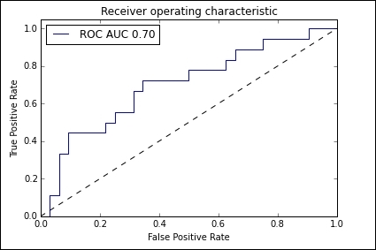
The ROC curve maps the true positive rates against the false positive rate for different threshold values. In the preceding diagram, this is represented by the dotted line. Once we have constructed the ROC curve, we calculate the number of positives, m_i, and the total number of instances, n_i, in each segment of the convex hull. The following formula is then used to calculate the calibrated feature values:

In this formula, c is the prior odds, that is, the ratio of the probability of the positive class over the probability of the negative class.

So far in our discussion on feature transformations, we assumed that we know all the values for every feature. In the real world, this is often not the case. If we are working with probabilistic models, we can estimate the value of a missing feature by taking a weighted average over all features values. An important consideration is that the existence of missing feature values may be correlated with the target variable. For example, data in an individual's medical history is a reflection of the types of testing that are performed, and this in turn is related to an assessment on risk factors for certain diseases.

If we are using a tree model, we can randomly choose a missing value, allowing the model to split on it. This, however, will not work for linear models. In this case, we need to fill in the missing values through a process of imputation. For classification, we can simply use the statistics of the mean, median, and mode over the observed features to impute the missing values. If we want to take feature correlation into account, we can construct a predictive model for each incomplete feature to predict missing values.

Since scikit-learn estimators always assume that all values in an array are numeric, missing values, either encoded as blanks, NaN, or other placeholders, will generate errors. Also, since we may not want to discard entire rows or columns, as these may contain valuable information, we need to use an imputation strategy to complete the dataset. In the following code snippet, we will use the Imputer class:

from sklearn.preprocessing import Binarizer, Imputer, OneHotEncoder
imp = Imputer(missing_values='NaN', strategy='mean', axis=0)
print(imp.fit_transform([[1, 3], [4, np.nan], [5, 6]]))

Here is the output:

Many machine learning algorithms require that features are standardized. This means that they will work best when the individual features look more or less like normally distributed data with near-zero mean and unit variance. The easiest way to do this is by subtracting the mean value from each feature and scaling it by dividing by the standard deviation. This can be achieved by the scale() function or the standardScaler() function in the sklearn.preprocessing() function. Although these functions will accept sparse data, they probably should not be used in such situations because centering sparse data would likely destroy its structure. It is recommended to use the MacAbsScaler() or maxabs_scale() function in these cases. The former scales and translates each feature individually by its maximum absolute value. The latter scales each feature individually to a range of [-1,1]. Another specific case is when we have outliers in the data. In these cases using the robust_scale() or RobustScaler() function is recommended.

Often, we may want to add complexity to a model by adding polynomial terms. This can be done using the PolynomialFeatures() function:

from sklearn.preprocessing import PolynomialFeatures
X=np.arange(9).reshape(3,3)
poly=PolynomialFeatures(degree=2)
print(X)
print(poly.fit_transform(X))

We will observe the following output: