
The hidden Markov model has numerous applications related to speech recognition, face identification (biometrics), and pattern recognition in pictures and video [7:3].
A hidden Markov model consists of a Markov process (also known as a Markov chain) for observations with a discrete time. The main difference with the Markov processes is that the states are not observable. A new observation is emitted with a probability known as the emission probability each time the state of the system or model changes.
There are now two sources of randomness:
- Transition between states
- Emission of an observation when a state is given
Let's reuse the boxes and balls example. If the boxes are hidden states (non-observable), then the user draws the balls whose color is not visible. The emission probability is the probability bik =p(ot= colork| qt=Si) to retrieve a ball of the color k from a hidden box I, as described in the following diagram:

The hidden Markov model for the balls and boxes example
In this example, we do not assume that all the boxes contain balls of different colors. We cannot make any assumptions on the order as defined by the transition aij. The HMM does not assume that the number of colors (observations) is identical to the number of boxes (states).
It must be kept in mind that the observations, in this case the color of the balls, are the only tangible data available to the experimenter. From this example, we can conclude that a formal HMM has three components:
- A set of observations
- A sequence of hidden states
- A model that maximizes the joint probability of the observations and hidden states, known as the Lambda model
A Lambda model, λ, is composed of initial probabilities π, the probabilities of state transitions as defined by the matrix A, and the probabilities of states emitting one or more observations:

Visualization of the HMM key components
This diagram illustrates that, given a sequence of observations, HMM tackles three problems known as canonical forms:
- CF1—evaluation: Evaluate the probability of a given sequence of observations Ot, given a model λ = (π, A, B)
- CF2—training: Identify (or learn) a model λ = (π, A, B) given a set of observations O
- CF3—decoding: Estimate the state sequence Q with the highest probability to generate a given set of observations O and a model λ
The solution to these three problems uses dynamic programming techniques. However, we need to clarify the notations prior to diving into the mathematical foundation of the hidden Markov model.
One of the challenges of describing the hidden Markov model is the mathematical notation that sometimes differs from author to author. From now on, we will use the following notation:
|
Description |
Formulation | |
|---|---|---|
|
N |
The number of hidden states | |
|
S |
A finite set of N hidden states |
S = {S0, S1, … SN-1} |
|
M |
The number of observation symbols | |
|
qt |
The state at time or step t | |
|
Q |
Time sequence of states |
Q = {q0, q1, … qn-1} = Q0:n-1 |
|
T |
The number of observations | |
|
ot |
The observation at time t | |
|
O |
A finite sequence of T observations |
O = {o0, o1, … oT-1} = O0:T-1 |
|
A |
The state transition probability matrix |
aji = p(qt+1=Si| qt=Sj) |
|
B |
The emission probability matrix |
bjk = p(ot=Ok| qt=Sj) |
|
π |
The initial state probability vector |
πi = p(q0=Sj) |
|
λ |
The hidden Markov model |
λ = (π, A, B) |
For convenience, let's simplify the notation of the sequence of observations and states using the following condensed form: p(O0:T, qt| λ) = p(O0, O1, … OT, qt| λ). It is quite common to visualize a hidden Markov model with a lattice of states and observations similar to our description of the boxes and balls examples, as shown here:

The formal HMM-directed graph
The state Si is observed as Ok at time t, before being transitioned to the state Sj observed as Om at the time t+1. The first step in the creation of our HMM is the definition of the class that implements the lambda model λ = (π, A, B) [7:4].
The three canonical forms of the hidden Markov model rely heavily on manipulation and operations on matrices and vectors. For convenience, let's define an HMMConfig class that contains the dimensions used in the HMM:
class HMMConfig(val _T: Int, val _N: Int, val _M: Int) extends ConfigThe input parameters for the class are:
_T: The number of observations_N: The number of hidden states_M: The number of observation symbols or features
Tip
Consistency with mathematical notation
The implementation uses _T (with respect to _N, _M) to represent programmatically the number of observations T (with respect to hidden states N and features M). As a general rule, the implementation reuses the mathematical symbols as much as possible. Although the practice does not always make the code elegant, it improves its readability.
The HMMConfig companion object defines the operations on ranges of index of matrix rows and columns. The foreach, foldLeft, and maxBy methods are regularly used in each of the three canonical forms:
object HMMConfig {
   def foreach(i: Int, f: Int => Unit): Unit = Range(0, i).foreach(f)
   def foldLeft(i: Int, f: (Double, Int) => Double, zero:Double) = Range(0, i).foldLeft(zero)(f)
   def maxBy(i: Int, f: Int => Double): Int = Range(0,i).maxBy(f)
   …
}
Note
Notation
The λ model in HMM should not be confused with the regularization factor discussed in the Ln roughness penalty section in Chapter 6, Regression and Regularization.
As mentioned earlier, the lambda model is defined as a tuple of the transition probability matrix A, emission probability matrix B, and the initial probability π. It is easily implemented as a case class, HMMLambda, using the Matrix class defined in the Matrix class section in Appendix A, Basic Concepts. The simplest constructor for the HMMLambda class is invoked in the case where the state-transition probability matrix, the emission probability matrix, and the initial states are known, as shown here:
class HMMLambda(val A: Matrix[Double], val B: Matrix[Double], var pi: DblVector, val numObs: Int) {
  def getT: Int = numObs
  def getN: Int = A.nRows
  def getM: Int = B.nCols
  val d1 = numObs -1
…
}
The implementation reflects the mathematical notation, with pi being the initial state probability, A the state transition matrix, and B the emission matrix. The numObs value is the number of observations in the sequence. The getT, getN, and getM methods are used to keep the implementation consistent with the initial configuration, HMMConfig. The section related to the training of HMM introduces a different constructor for HMMLambda using the configuration as a parameter.
The initial probabilities are unknown, and therefore, initialized with a random generator of values [0, 1].
The two other components of the HMM are the sequence of observations and the sequence of hidden states.
The canonical forms of the HMM are implemented through dynamic programming techniques. These techniques rely on variables that define the state of the execution of the HMM for any of the canonical forms:
Alpha(the forward variable): The probability of observing the first t < T observations for a specific state at Si for the observation t, αt(i) = p(O0:t, qt=Si|λ)Beta(the backward variable): The probability of observing the remainder of the sequence qt for a specific state βt(i) = p(Ot+1:T-1|qt=Si,λ)Gamma: The probability of being in a specific state given a sequence of observations and a model γt(i) =p(qt=Si|O0:T-1, λ)Delta: The sequence to have the highest probability path for the first i observations defined for a specific test δt(i)Qstar: The optimum sequence q* of states Q0:T-1DiGamma: The probability of being in a specific state at t and another defined state at t+1 given the sequence of observations and the model γt(i,j) =p(qt=Si,qt+1=Sj|O0:T-1, λ)
Each of the parameters is described in the section related to each canonical form. Let's create a class HMMState that encapsulates the variables used in the implementation of the three canonical cases.
For convenience, all the parameters related to the three canonical cases and listed in the previous notation section are encapsulated into a single outer class, HMMState:
class HMMState(lambda: HMMLambda, maxIters:Int) extends Config {
  val delta = Matrix[Double]( lambda.getT, lambda.get N)  // δt(i)

  object QStar { … } //q*
  object DiGamma { … } // γt(i, j)
  object Gamma { … }  // γt(i)
}
Once again, we use the same notation as for the configuration of the HMM; lambda.getT, being the number of observations, and lambda.getN, the number of hidden states. The HMM state parameters have self-descriptive names that strictly follow the notation introduced earlier. The ![]() model, the HMM state, and the sequence of observations are all the elements needed to implement the three canonical cases.
model, the HMM state, and the sequence of observations are all the elements needed to implement the three canonical cases.
The Gamma and DiGamma singletons are used and described in the evaluation canonical form. The DiGamma singleton is described as part of the Viterbi algorithm to extract the sequence of states with the highest probability given a ![]() model and a set of observations.
model and a set of observations.
The execution of any of the three canonical forms relies on dynamic programming techniques (refer to the Overview of dynamic programming section in Appendix A, Basic Concepts) [7:5]. The simplest of the dynamic programming techniques is a single traversal of the observations/state chain.
Therefore, it makes sense to define a base class, HMMModel, that has all the algorithms that manipulate the ![]() model,
model, lambda, and the observed states, obs:
abstract class HMMModel(lambda: HMMLambda, obs: Array[Int])The list of dynamic-programming-related algorithms used in any of the three canonical forms is visualized through the class hierarchy of our implementation of the HMM:

Scala classes' hierarchy for HMM (UML class diagram)
Each class is described as needed in the description of the three canonical forms of HMM. It is time to dive into the implementation details of each of the canonical forms, starting with the evaluation.
The objective is to compute the probability (or likelihood) of the observed sequence Ot given a ![]() model. A dynamic programming technique is used to break down the probability of the sequence of observations into two probabilities:
model. A dynamic programming technique is used to break down the probability of the sequence of observations into two probabilities:
The likelihood is computed by marginalizing over all the hidden states [7:6]{Si}:

If we use the notation introduced in the previous chapter for alpha and beta variables, the probability for the observed sequence Ot given a ![]() model can be expressed as:
model can be expressed as:
The product of the probabilities α and β can potentially underflow. Therefore, it is recommended to use the log of the probabilities instead of the probabilities.
The computation of the probability of observing a specific sequence given a sequence of hidden states and a ![]() model relies on a two-pass algorithm. The alpha algorithm consists of the following steps:
model relies on a two-pass algorithm. The alpha algorithm consists of the following steps:
- Compute the initial alpha value [M1]. The value is then normalized by the sum of alpha values across all the hidden states [M2].
- Compute the alpha value iteratively for the time 0 to time t, then normalize by the sum of alpha values for all states [M3].
- The final step is the computation of the log of the probability of observing the sequence [M4].
For those with some inclination toward mathematics, computation of the alpha matrix is defined in the following information box. Each formula has an identifier [Mx], which is referenced in the Scala source code implementing it.


Let's look at the implementation of the alpha class in Scala, using the referenced number of the mathematical expressions of the alpha class. The alpha and beta values have to be normalized [M3], and therefore, we define a base class, Pass, for the alpha and beta algorithms that implements the normalization:
class Pass(_lambda: HMMLambda, _obs: Array[Int]) extends HMMModel(_lambda, _obs) {  //1
   var alphaBeta: Matrix[Double] = _
   val ct = Array.fill(lambda.getT)(0.0) //2

   def normalize(t: Int): Unit = {
     ct.update(t, foldLeft(lambda.getN, (s, n) => s + alphaBeta(t, n))) //3
     alphaBeta /= (t, ct(t))
   }
}
As with any algorithm used in the hidden Markov model, the Pass base class of the alpha and beta classes is a composition of the attributes of the model (HMMLambda), the computation parameters (HMMParams), and the sequence of observations obs (line 1). The alphaBeta matrix represents either the alpha or beta matrix manipulated in the subclasses (line 2). The scale factor, ct, is computed as the summation of the alpha or beta row matrix over all the states using a fold (line 3).
The computation of the alpha variable in the Alpha class follows the same computation flow as defined in the mathematical expression:
class Alpha(lambda: HMMLambda, obs: Array[Int]) extends Pass(lambda, obs)The alpha value is initialized [M1] (line 4), then normalized [M2] using the current sequence order (line 5). The value of alpha is then updated [M3] by summation of the previous alpha value at t-1 and the transition from the state j to the state i (line 6), as shown here:
Import HMMConfig._
val alpha = {
  alphaBeta = lambda.initAlpha(obs) //4
  normalize(0)  //5
  sumUp //6
}

def sumUp: Double = { //[M2]
  foreach(lambda.getT, t => {
    updateAlpha(t) //7
    normalize(t) //8
  })
  foldLeft(lambda.getN, (s, k) => s + alphaBeta(lambda.dim_1, k))
}

def updateAlpha(t: Int): Unit =
  HMMConfig.foreach(lambda.getN, i =>
    alphaBeta += (t,i,lambda.alpha(alphaBeta(t-1,i),i,obs(t)))
   )
}
The value of alpha is updated by the updateAlpha method (line 7) before normalization (line 8). The implementation that relies on the fold method is omitted, but can be easily written.
Finally, the computation of the logarithm of the probability to observe a specific sequence, given the sequence of states and a predefined ![]() model, [M4] can be performed by the following code (line
model, [M4] can be performed by the following code (line 9):
def logProb: Double = foldLeft(lambda.getT, (s, t)
                    => s + Math.log(ct(t)), Math.log(alpha))//9
The method computes the logarithm of the probability instead of the probability itself. The summation of the logarithm of probabilities is less likely to cause an underflow than the product of probabilities.
The recursive computation of beta values is similar to the Alpha class except that the iteration executes backward on the sequence of states.
The implementation of Beta is similar to the alpha class:
- Compute [M5] and normalize [M6] the value of beta at t=0 across states.
- Compute and normalize iteratively the beta at the time T-1 to t updated from its value at t+1 [M7].

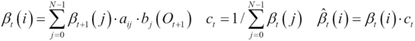
The definition of the class for the Beta class is identical to the Alpha class:
class Beta(lambdaB: HMMLambda, _obs: Array[Int]) extends Pass(lambdaB, _obs)The implementation of the Beta class is similar to the Alpha class with computation (line 1) and normalization (line 2) of beta at t=0. As expected, the summation routine sumUp (line 3) is implemented as updating and normalizing beta at the time t, as shown here:
val complete = { //4
   alphaBeta = Matrix[Double](lambda.getT, lambda.getN)
   alphaBeta += (lambda.dim_1, 1.0) //1
   normalize(lambda.dim_1)  //2
   sumUp; true
}

def sumUp: Unit = //3
  (lambda.getT-2 to 0 by -1).foreach( t =>{
    updateBeta(t)
    normalize(t)
})

def updateBeta(t: Int): Unit =
  foreach(lambda.config.getN, i => {
    alphaBeta += (t, i, lambda.beta(alphaBeta(t+1, i), i, obs(t+1)))
})
The recursive method updates and normalizes the beta matrix by traversing the sequence of observations backward from before the last observation to the first. Contrary to the Alpha class, the Beta class does not generate an output value. Therefore, we need to flag the state of the class using a ready Boolean value, which is set to true if the instantiation succeeds and false otherwise.
Note
Constructors
The alpha and beta values are computed within the constructors of their respective class, so no public or protected method needs to verify if these values are already computed. The design pattern reduces the complexity of implementation by ensuring that a class instance has only one state: computation completed.
What is the value of a model if it cannot be created? The next canonical form CF2 leverages dynamic programming and recursive functions to extract the ![]() model.
model.
The objective of this canonical form is to extract the ![]() model given a set of observations and a sequence of states. It is similar to the training of a classifier. The simple dependency of a current state on the previous state enables an implementation using an iterative procedure, known as the Baum-Welch estimator or expectation-maximization (EM).
model given a set of observations and a sequence of states. It is similar to the training of a classifier. The simple dependency of a current state on the previous state enables an implementation using an iterative procedure, known as the Baum-Welch estimator or expectation-maximization (EM).
At its core, the algorithm has three steps and an iterative method, similar to the evaluation canonical form:
- Compute the probability π (the gamma value at t=0) [M9].
- Compute and normalize the state's transition probabilities matrix A [M10].
- Compute and normalize the matrix of emission probabilities B [M11].
- Repeat steps 2 and 3 until the change of likelihood is insignificant.
The algorithm uses the digamma and summation gamma variables defined in the HMMConfig class.


The Baum-Welch algorithm requires the following three inputs:
-
The
 model,
 _lambda, initialized with random values uniformly distributed - The current state of the training,
state - The labeled observed data,
_obsIdx
The implementation of the Baum-Welch algorithm illustrates the elegance and conciseness of the Scala programming language. The constructor requires a fourth parameter to describe the minimum rate of change of the estimate of the likelihood between iterative calls, as shown in the following code snippet:
class BaumWelchEM config: HMMConfig, obs: Array[Int], numIters: Int,eps: Double) extends HMMModel(HMMLambda(config), obs) {
  val state = HMMState(lambda, numIters)
}
The ![]() model has to be initialized with the configuration parameters (number of observations, number of states, and number of symbols). The matrices
model has to be initialized with the configuration parameters (number of observations, number of states, and number of symbols). The matrices A and B and the initial state probabilities pi are initialized with a uniform random generator [0, 1], Matrix.fillRandom, as shown here:
object HMMLambda {
  def apply(config: HMMConfig): HMMLambda = {
    val A = Matrix[Double](config._N)
    A.fillRandom(0.0)
    val B = Matrix[Double](config._N, config._M)
    B.fillRandom(0.0)
    val pi = Array.fill(config._N)(Random.nextDouble)
    new HMMLambda(A, B, pi, config._T)
   }
The maximum likelihood, maxLikelihood, is computed as part of the constructor to ensure a consistent state:
var likelihood = frwrdBckwrdLattice
Range(0, state.maxIters) find( _ => {
   lambda.estimate(state, obs)   //1
   val _likelihood = frwrdBckwrdLattice  //2
   val diff = likelihood - _likelihood  //3
   likelihood = _likelihood
   diff < eps  //4
}) match {
   case Some(index) => maxLikelihood
…
The computation of the likelihood requires the estimation of the transition matrix A and emission matrix B (line 1). The training process iterates by traversing the lattice forward and backward until the likelihood reaches a local or global maximum. The ![]() model is updated using the
model is updated using the estimate method (line 1). The method computes the likelihood of the sequence of states (line 2) and then compares it with the likelihood computed in the previous iteration (line 3). The method exits if the difference between two consecutive likelihood values meets the convergence criteria eps (line 4).
The estimate method of the HMMLambda class updates the ![]() model (
model (A, B, and pi):
def estimate(state: HMMState, obsIdx: Array[Int]): Unit = {
  pi = Array.tabulate(config._N)(i => state.Gamma(0, i) )
  HMMConfig.foreach(config._N, i => {

  var denominator = state.Gamma.fold(dim_1, i)
  HMMConfig.foreach(config._N, k =>
     A += (i, k, state.DiGamma.fold(dim_1, i, k)/denominator)
  )
  denominator = state.Gamma.fold(config._T, i)
  HMMConfig.foreach(config._N, k => B += (i, k, state.Gamma.fold(config._T, i, k, obsIdx)/denominator))
})
The core of the Baum-Welch expectation maximization is the iterative forward and backward update of the lattice of states and observations between time t and t+1. The lattice-based iterative computation is illustrated in the following diagram:

Visualization of HMM graph lattice for the Baum-Welch algorithm
The iteration across the lattice is implemented by the frwrdBckwrdLattice method (line 2). The lattice is traversed ahead using the Alpha instance class (line 1), and backward using the Beta instance class (line 2):
def frwrdBckwrdLattice: Double  = {
   val _alpha = Alpha(lambda, obs).alpha //1
   val _beta = Beta(lambda, obs) //2
   val a = _alpha.alphaBeta
   val b = _beta.alphaBeta
   Gamma.update(a, b)  //3
   DiGamma.update(a, b, A, B, obs) //4
   _alpha.alpha
}
The method returns the alpha coefficient and computes the new values for the Gamma (line 3) vector and DiGamma (line 4) matrix. These HMMState methods are omitted for the sake of clarity.
This last canonical form consists of extracting the most likely sequence of states {qt} given a set of observations Ot and a ![]() model. Solving this problem requires, once again, a recursive algorithm.
model. Solving this problem requires, once again, a recursive algorithm.
The extraction of the best state sequence (the sequence of state that has the highest probability) is very time consuming. An alternative consists of applying a dynamic programming technique to find the best sequence {qt} through iteration. The algorithm is known as the Viterbi algorithm. Given a sequence of states {qt} and sequence of observations {oj}, the probability δt(i) for any sequence to have the highest probability path for the first T observations is defined for the state St [7:7].


The constructor of the Viterbi algorithm, ViterbiPath, is similar to the algorithms of the first two canonical forms, and therefore, inherits HMMInference. The purpose of the Viterbi algorithm is to compute the optimum sequence given a set of observations and a ![]() model by maximizing the delta,
model by maximizing the delta, maxDelta:
class ViterbiPath(_lambda: HMMLambda, _state: HMMState, _obs: Array[Int]) extends HMMInference(_lambda, _state, _obs) {
  val maxDelta = recurse(lambda.getT, 0)
  …
}
The recursive method that implements [M14] and [M15] steps is invoked by the constructor:
def recurse(t: Int, j: Int): Double = {
  var maxDelta = initial((t, j)) //1
  if( maxDelta == -1.0) {
    if(t != obs.size) {
        maxDelta = maxBy(lambda.getN, //2 [M14]
           s => recurse(t-1, s)* lambda.A(s, j)* lambda.B(j, obs(t))
         )
       val idx =maxBy(lambda.getT, i =>recurse(t-1 ,i)*lambda.A(i,j))  //3 [M14]

       state.psi += (t, j, idx) //4
       state.delta += (t, j, maxDelta) //5
     }
     else {  //6
       maxDelta = 0.0
       val index =maxBy(lambda.getN, i => {
          val delta = recurse(t-1 ,i)
          if( delta > maxDelta) maxDelta = delta
          delta
       })
       state.QStar.update(t, index) //7
     }
   }
   maxDelta
}
Once initialized (line 1), the maximum value of delta, maxDelta, is computed recursively by applying the formula [M14] at each state, s, using Scala's maxBy method (line 2). Next, the index of the column of the transition matrix A corresponding to the maximum of delta is computed (line 3). The last step is to update the matrix psi (line 4) (with respect to delta (line 5)). Once the step t reaches the maximum number of observation labels (line 6), the optimum sequence of states q* is computed [M15] (line 7). Ancillary methods are omitted.
This implementation of the decoding form of the hidden Markov model completes the description of the hidden Markov model and its implementation in Scala. Now, let's put this knowledge into practice.
The main class HMM implements the three canonical forms. A view bound to an array of integers is used to parameterize the HMM class. We assume that a time series of continuous or pseudocontinuous values is converted (or categorized) into discrete symbol values.
The @specialized annotation ensures that the byte code is generated for the Array[Int] primitive without executing the conversion implicitly declared by the bound view. The HMM can be potentially used as part of a computation workflow, and therefore, has to implement the pipe operator (PipeOperator).
There are two different constructors for the HMM class. The first constructor uses the ![]() model as input (evaluation (CF1) and decoding (CF3)):
model as input (evaluation (CF1) and decoding (CF3)):
class HMM[@specialized T <% Array[Int]](lambda: HMMLambda, form: HMMForm, maxIters: Int) (implicit f: DblVector => T) extends PipeOperator[T, HMMPredictor] {
  val state = HMMState(lambda, maxIters)
….
}
The HMMForm enumerator is used to specify the canonical form of the HMM solution:
object HMMForm extends Enumeration {
type HMMForm = Value
val EVALUATION,DECODING = Value
}
The conversion of DblVector to a type T is required only if the evaluation and decoding canonical form uses actual observation values as argument. The f function is then used to discretize the double values into a sequence of index of the observations.
The HMMPredictor type consists of a tuple log probability (or likelihood) of observations and index of sequence of observations:
type HMMPredictor = (Double, Array[Int])The HMM has three canonical forms instead of the two forms of most classifiers.
The second canonical form, training, is implemented by defining a second constructor for the HMM class, as follows:
object HMM {
  def apply[T <% Array[Int]](config: HMMConfig, obs: Array[Int], form: HMMForm, maxIters: Int, eps: Double)
                     (implicit f: DblVector => T): HMM[T] = {
    val baumWelchEM = new BaumWelchEM(config, obs, maxIters, eps)
    new HMM[T](baumWelchEM.lambda, form, maxIters)
  }
}
The decode (with respect to evaluate) method implements the third (with respect to the first) canonical form of HMM. Both methods take a sequence of indices for observations as an argument.
  def decode(obsIdx: Array[Int]): HMMPredictor = (ViterbiPath(lambda, state, obsIdx).maxDelta, state.QStar())
  def evaluate(obsIdx: Array[Int]): HMMPredictor = (-Alpha(lambda, obsIdx).logProb, obsIdx)
}
The data transformation |> encapsulates the evaluation and decoding forms in order to preserve its meaning. The observation, obs, is automatically converted into a sequence of indices to each observation (line 1) by the DblVector => T discretization function, which is an implicit parameter of the HMM class.
def |> : PartialFunction[DblVector, HMMPredictor] = {
  case obs: DblVector if(obs != null && obs.size > 2) => {
    form match {
      case EVALUATION => evaluate(obs)  //1
      case DECODING => decode(obs)  //1
    }
…
Tip
Normalized probabilities input
You need to make sure that the input probabilities for the ![]() model for evaluation and decoding canonical forms are normalized—the sum of the probabilities of all the states for the π vector and A and B matrices are equal to 1. This validation code is omitted in the example code.
model for evaluation and decoding canonical forms are normalized—the sum of the probabilities of all the states for the π vector and A and B matrices are equal to 1. This validation code is omitted in the example code.
Our test case is to train an HMM to predict the sentiment of investors as measured by the weekly sentiment survey of the members of the American Association of Individual Investors (AAII) [7:8]. The goal is to compute the transition probabilities matrix A, the emission probabilities matrix B, and the steady state probability distribution π, given the observations and hidden states (training canonical form).
We assume that the change in investor sentiments is independent of time, as required by the hidden Markov model.
The AAII sentiment survey grades the bullishness on the market in terms of percentage:

The weekly AAII market sentiment (reproduced by courtesy from AAII)
The sentiment of investors is known as a contrarian indicator of the future direction of the stock market. Refer to the Terminology section in Appendix A, Basic Concepts.
Let's select the ratio of percentage of investors that are bullish over the percentage of investors that are bearish. The ratio is then normalized. The following table lists this:
|
Time |
Bullish |
Bearish |
Neutral |
Ratio |
Normalized ratio |
|---|---|---|---|---|---|
|
t0 |
0.38 |
0.15 |
0.47 |
2.53 |
1.0 |
|
t1 |
0.41 |
0.25 |
0.34 |
1.68 |
0.53 |
|
t2 |
0.25 |
0.35 |
0.40 |
0.71 |
0.0 |
|
…. |
The sequence of non-normalized observations (ratio of bullish sentiment over bearish sentiment) is defined in a CSV file as follows:
final val OBS_PATH = "resources/data/chap7/obs.csv"

final val NUM_SYMBOLS = 6
final val NUM_STATES = 5
final val EPS = 1e-3
final val MAX_ITERS = 250


val srcObs =  Source.fromFile(OBS_PATH)
val obs = srcObs.getLines.map(_.toDouble)).toSeq //1
val config = new HMMConfig(obs.size, NUM_STATES, NUM_SYMBOLS)
val min = obs.min
val delta = obs.max - min
val obsSeq = obs.map( x => (x - min)/delta) //2
                .map(x =>(x*NUM_SYMBOLS).floor.toInt) //3
HMM[Array[Int]](config,obsSeq,EVALUATION,MAX_ITERS,EPS) match {
  case Some( hmm) => //4
     Display.show(s"Lambda: ${hmm.getModel.toString}", logger)
   …
}
The sequence of observations is loaded from the CSV file (line 1) before being normalized (line 2). The discretization converts the normalized bullish sentiment/bearish sentiment ratio in six levels (integers) [0,-5] (line 3). The instantiation of the HMM class for the ratio levels (Array[Int]) generates the ![]() model (
model (A, B, and pi) (line 4).
The following is a state-transition matrix:
|
A |
1 |
2 |
3 |
4 |
5 |
|---|---|---|---|---|---|
|
1 |
0.090 |
0.026 |
0.056 |
0.046 |
0.150 |
|
2 |
0.094 |
0.123 |
0.074 |
0.058 |
0.0 |
|
3 |
0.093 |
0.169 |
0.087 |
0.061 |
0.056 |
|
4 |
0.033 |
0.342 |
0.017 |
0.031 |
0.147 |
|
5 |
0.386 |
0.47 |
0.314 |
0.541 |
0.271 |
The emission matrix is as follows:
|
B |
1 |
2 |
3 |
4 |
5 |
6 |
|---|---|---|---|---|---|---|
|
1 |
0.203 |
0.313 |
0.511 |
0.722 |
0.264 |
0.307 |
|
2 |
0.149 |
0.729 |
0.258 |
0.389 |
0.324 |
0.471 |
|
3 |
0.305 |
0.617 |
0.427 |
0.596 |
0.189 |
0.186 |
|
4 |
0.207 |
0.312 |
0.351 |
0.653 |
0.358 |
0.442 |
|
5 |
0.674 |
0.520 |
0.248 |
0.294 |
0.259 |
0.03 |
The evaluation form of the hidden Markov model is very suitable for filtering data for discrete states. Contrary to time series filters such as the Kalman filter introduced in the The Kalman filter section in Chapter 3, Data Preprocessing, HMM requires data to be somewhat stationary in order to create a reliable model. However, the hidden Markov model overcomes some of the limitations of analytical time series analysis. Filters and smoothing techniques assume that the noise (frequency mean, variance, and covariance) is known and usually follows a Gaussian distribution. The hidden Markov model does not have such a restriction. Moreover, moving averaging techniques, discrete Fourier transforms, and generic Kalman filters require the states to be continuous with linear dependencies, although the extended Kalman filter can approximate nonlinear states.