
The popularity of neural networks surged in the 90s. They were seen as the silver bullet to a vast number of problems. At its core, a neural network is a nonlinear statistical model that leverages the logistic regression to create a nonlinear distributed model. The concept of artificial neural networks is rooted in biology, with the desire to simulate key functions of the brain and replicate its structure in terms of neurons, activation, and synapses.
In this chapter, you will move beyond the hype and learn:
The idea behind artificial neural networks was to build mathematical and computational models of the natural neural network in the brain. After all, the brain is a very powerful information processing engine that surpasses computers in domains such as learning, inductive reasoning, prediction and vision, and speech recognition.
In biology, a neural network is composed of groups of neurons interconnected though synapses [9:1], as shown in the following image:

Neuroscientists have been especially interested in understanding how the billions of neurons in the brain can interact to provide human beings with parallel processing capabilities. The 60s saw a new field of study emerging, known as connectionism. Connectionism marries cognitive psychology, artificial intelligence, and neuroscience. The goal was to create a model for mental phenomena. Although there are many forms of connectionism, the neural network models have become the most popular and the most taught of all connectionism models [9:2].
Biological neurons communicate through electrical charges known as stimuli. This network of neurons can be represented as a simple schematic, as follows:

This representation categorizes groups of neurons as layers. The terminology used to describe the natural neural networks has a corresponding nomenclature for the artificial neural network.
|
The biological neural network |
The artificial neuron network |
|---|---|
|
Axon |
Connection |
|
Dendrite |
Connection |
|
Synapse |
Weight |
|
Potential |
Weighted sum |
|
Threshold |
Bias weight |
|
Signal, Stimulus |
Activation |
|
Group of neurons |
Layer of neurons |
In the biological world, stimuli do not propagate in any specific direction between neurons. An artificial neural network can have the same degree of freedom. The artificial neural networks most commonly used by data scientists, have a predefined direction: from the input layer to output layers. These neural networks are known as FFNN.
In the previous chapter, you learned that support vector machines have the ability to formulate the training of a model as a nonlinear optimization for which the objective function is convex. A convex objective function is fairly straightforward to implement. The drawback is that the kernelization of the SVM may result in a large number of basis functions (or model dimensions). Refer to the The Kernel trick section under The support vector machine (SVM) in Chapter 8, Kernel Models and Support Vector Machines.
One solution is to reduce the number of basis functions through parameterization, so these functions can adapt to different training sets. Such an approach can be modeled as a FFNN, known as the multilayer perceptron [9:3].
The linear regression can be visualized as a simple connectivity model using neurons and synapses, as follows:

A two-layer neural network
The feature x0=+1 is known as the bias input (or bias element), which corresponds to the intercept in the classic linear regression.
As with support vector machines, linear regression is appropriate for observations that can be linearly separable. The real world is usually driven by a nonlinear phenomena. Therefore, the logistic regression is naturally used to compute the output of the perceptron. For a set of input variable x = {xi}0,n and the weights w={wi}1,n, the output y is computed as:
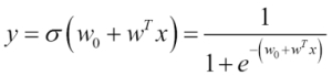
An FFNN can be regarded as a stack of layers of logistic regression with the output layer as a linear regression.
The value of the variables in each hidden layer is computed as the sigmoid of the dot product of the connection weights and the output of the previous layer. Although interesting, the theory behind artificial neural networks is beyond the scope of this book [9:4].