
Support vector machines can be applied to classification, anomalies detection, and regression problems. Let's dive into the support vector classifiers first.
The first classifier to be evaluated is the binary (2-class) support vector classifier. The implementation uses the LIBSVM library created by Chih-Chung Chang and Chih-Jen Lin from the National Taiwan University [8:9].
The library was originally written in C and ported to Java. It can be downloaded from http://www.csie.ntu.edu.tw/~cjlin/libsvm as a .zip or tar.gzip file. The library includes the following classifier modes:
- Support vector classifiers (C-SVC, υ-SVC, and one-class SVC)
- Support vector regression (υ-SVR and ε-SVR)
- RBF, linear, sigmoid, polynomial, and precomputed kernels
LIBSVM has the distinct advantage of using Sequential Minimal Optimization (SMO), which reduces the time complexity of a training of n observations to O(n2). LIBSVM documentation covers both the theory and implementation of hard and soft margins and is available at http://www.csie.ntu.edu.tw/~cjlin/papers/guide/guide.pdf.
Tip
Why LIBSVM?
There are alternatives to the LIBSVM library for learning and experimenting with SVM. David Soergel from the University of Berkeley refactored and optimized the Java version [8:10]. Thorsten Joachims' SVMLight [8:11] Spark/MLlib 1.0 includes two Scala implementations of SVM using resilient distributed datasets (refer to the Apache Spark section of Chapter 12, Scalable Frameworks). However, LIBSVM is the most commonly used SVM library.
The implementation of the different support vector classifiers and the support vector regression in LIBSVM is broken down into the following five Java classes:
svm_model: This defines the parameters of the model created during trainingsvm_node: This models the element of the sparse matrix Q, used in the maximization of the marginssvm_parameters: This contains the different models for support vector classifiers and regressions, the five kernels supported in LIBSVM with their parameters, and the weights vectors used in cross-validationsvm_problem: This configures the input to any of the SVM algorithm (number of observations, input vector data x as a matrix, and the vector of labels y)svm: This implements algorithms used in training, classification, and regression
The library also includes template programs for training, prediction, and normalization of datasets.
Tip
The LIBSVM Java code
The Java version of LIBSVM is a direct port of the original C code. It does not support generic types and is not easily configurable (the code uses switch statements instead of polymorphism). For all its limitations, LIBSVM is a fairly well-tested and robust Java library for SVM.
Let's create a Scala wrapper to the LIBSVM library to improve its flexibility and ease of use.
The implementation of the support vector machine algorithm uses the design template for classifiers (refer to the Design template for classifier section in Appendix A, Basic Concepts).
The key components of the implementation of an SVM are as follows:
- A model
SVMModelof the typeModel, which is initialized through training during the instantiation of the classifier. The model class is an adapter to thesvm_modelstructure defined in LIBSVM. - A predictive or classification routine is implemented as a data transformation extending the
PipeOperatortrait. - The support vector machine class
SVMhas three parameters: the configuration wrapper of the typeSVMConfig, the features/time series of the typeXTSeries, and the target or labeled valuesDblVector. - The configuration (the type
SVMConfig) consists of three distinct elements:SVMExecutionthat defines the execution parameters such as maximum number of iterations or convergence criteria,SVMKernelthat specifies the kernel function used during training, andSVMFormulationthat defines the formula (C, epsilon, or nu) used to compute a nonseparable case for the support vector classifier and regression.
The key software components of the support vector machine are described in the following UML class diagram:

LIBSVM exposes a large number of parameters for the configuration and execution of any of the SVM algorithms. Any SVM algorithm is configured with three categories of parameters, which are as follows:
- Formulation (or type) of the SVM algorithms (multiclass classifier, one-class classifier, regression, and so on) using the
SVMFormulationclass - The kernel function used in the algorithm (the RBF kernel, Sigmoid kernel, and so on) using the
SVMKernelclass - Training and execution parameters (convergence criteria, number of folds for cross-validation, and so on) using the
SVMExecutionclass
The instantiation of the configuration consists of initializing the LIBSVM parameter, param, by the SVM type, kernel, and the execution context selected by the user.
Each of the SVM parameters case class extends the generic trait, SVMConfigItem:
trait SVMConfigItem { def update(param: svm_parameter): Unit }
The classes inherited from SVMConfigItem are responsible for updating the list of the SVM parameters, svm_parameter, defined in LIBSVM. The update method encapsulates the configuration of the LIBSVM.
The formulation of the SVM algorithm is defined by classes implementing the SVMFormulation trait:
sealed trait SVMFormulation extends SVMConfigItem {
  def update(param: svm_parameter): Unit
}
The list of formulation for the SVM (C, nu, and eps for regression) is completely defined and known. Therefore, the hierarchy should not be altered and the SVMFormulation trait has to be declared sealed. Here is an example of the SVM formulation class, CSVCFormulation, which defines the C-SVM model:
class CSVCFormulation (c: Double) extends SVMFormulation {
  override def update(param: svm_parameter): Unit = {
     param.svm_type = svm_parameter.C_SVC
     param.C = c
  }
}
The other SVM formulation classes, NuSVCFormulation, OneSVCFormulation, and SVRFormulation, implement the υ-SVM, 1-SVM, and ε-SVM respectively for regression models.
Next, you need to specify the kernel functions by defining and implementing the SVMKernel trait:
sealed trait SVMKernel extends SVMConfigItem {
   def update(param: svm_parameter): Unit
}
Once again, there are a limited number of kernel functions supported in LIBSVM. Therefore, the hierarchy of kernel functions is sealed. The following code snippet configures the radius basis function kernel, RbfKernel, as an example of definition of the kernel definition class:
class RbfKernel(gamma: Double) extends SVMKernel {
  override def update(param: svm_parameter): Unit = {
    param.kernel_type = svm_parameter.RBF
    param.gamma = gamma
…
The fact that the LIBSVM Java byte code library is not very extensible does not prevent you from defining a new kernel function in the LIBSVM source code. For example, the Laplacian kernel can be added with the following steps:
- Create a new kernel type in
svm_parameter, such assvm_parameter.LAPLACE = 5. - Add the kernel function name to
kernel_type_tablein thesvmclass. - Add
kernel_type != svm_parameter.LAPLACEto thesvm_check_parametermethod. - Add the implementation of the kernel function for two values in
svm.kernel_function (java code):case svm_parameter.LAPLACE: double sum = 0.0; for(int k = 0; k < x[i].length; k++) { final double diff = x[i][k].value - x[j][k].value; sum += diff*diff; } return Math.exp(-gamma*Math.sqrt(sum)); - Add the implementation of the Laplace kernel function in the
svm.k_functionmethod by modifying the existing implementation of RBF (distanceSqr). - Rebuild the
libsvm.jarfile
The SVMExecution class defines the configuration parameters for the execution of the training of the model, namely, the convergence factor, eps for the optimizer, the size of the cache cacheSize, and the number of folds, nFolds used during cross-validation:
class SVMExecution(cacheSize: Int, eps: Double, nFolds: Int) extends SVMConfigItem {
  override def update(param: svm_parameter): Unit = {
    param.cache_size = cacheSize
    param.eps = eps
  }
}
The cross-validation is performed only if the nFolds value is greater than 1.
We are finally ready to create the configuration class, SVMConfig, which hides and manages all of the different configuration parameters:
class SVMConfig(formula: SVMFormulation, kernel: SVMKernel,exec: SVMExecution) {
   val param = new svm_parameter
   formula.update(param)
   kernel.update(param)
   exec.update(param)
}
The instantiation of SVMConfig initialized the internal LIBSVM list of configuration parameters through a sequence of update calls.
Next, let's implement the first support vector classifier for the two-class problems. As with any other data transformation, the parameterized class SVM implements the PipeOperator, as follows:
class SVM[T <% Double](config: SVMConfig, xt: XTSeries[Array[T]], labels: DblVector) extends PipeOperator[Array[T], Double] {
  type Feature = Array[T]
  type SVMNodes = Array[Array[svm_node]]
This class has the same parameters as other classifiers presented in the previous chapters: a configuration, config, an input time series, xt, and labeled data, labels. The types are added for convenience. The internal types, Feature and SVMNodes, are added for convenience.
The LIBSVIM type, svm_node, is the indexed value of an element of the feature vector in a particular observation:
public class svm_node implements java.io.Serializable {
   public int index;
   public double value;
}
The type SVMNodes defined in the scope of SVM class is the representation of a two-dimensional array of features vector elements by observations. The next step is to implement the training procedure. The training is executed during the instantiation of the SVM class. The SVM model, SVMModel, is defined as a tuple or pair (svmmodel, accuracy) with the following:
- The
svmmodelis the model defined in LIBSVM accuracycomputed during an N-folds cross-validation if the number of folds,nFolds, has been set as one of the parameters ofSVMExecution
Consider the following code:
class SVMModel(val svmmodel: svm_model, val accuracy: Double) extends Model
The instantiation of SVC is hidden from the client code. It is executed during the instantiation of the class, so a client code does not have to be aware of the LIBSVM types. Consider the following code:
val model: Option[SVMModel] = {
  val problem = new svm_problem  //1
  problem.l = xt.size;
  problem.y = labels
  problem.x = new SVMNodes(xt.size)

  val dim = dimension(xt)
  xt.zipWithIndex.foreach( xt_i => {  //2
     val svm_col = new Array[svm_node](dim)
     xt_i._1.zipWithIndex
            .foreach(xi =>  {
                val node = new svm_node
                node.index= xi._2
                node.value = xi._1
                svm_col(xi._2) = node
             })
     problem.x(xt_i._2) = svm_col
   })
  Some(svm.svm_train(problem, config.param, accuracy(problem))//3
}
The first step in the creation of the model is to define the SVM problem, problem, in the context of LIBSVM (line 1): length of the time series, labeled data, and input observations. The time series has to be converted into the LIBSVM internal class, svm_nodes (line 2), to complete the initialization of the problem. The Scala method, zipWithIndex, is used to access the index of each observation (time series entry). Finally, the model and the computed accuracy are returned as a tuple (line 3) after processing by the svm_train training method.
The accuracy is the ratio of true positive plus the true negative over the size of the test sample (refer to the Key metrics section of Chapter 2, Hello World!). It is computed through cross-validation only if the number of folds is initialized in the SVMExecution configuration class as greater than 1. Practically, the accuracy is computed by invoking the cross-validation method, svm_cross_validation, in the LIBSVM package, and then computing the ratio of the number of predicted values that match the labels over the total number of observations. Here is the essential part of the implementation of accuracy(problem: svm_problem):
val target = new Array[Double](labels.size)
svm.svm_cross_validation(problem, config.param, config.exec.nFolds, target)
val rawAccuracy = target.zip(labels)
                  .filter(z => Math.abs(z._1-z._2) < config.eps)
rawAccuracy.size.toDouble/labels.size
The Scala filter weeds out the observations that were poorly predicted. This minimalist implementation is good enough to start exploring the support vector classifier.
The first evaluation consists of understanding the impact of the penalty factor C to the margin in the generation of the classes. Let's implement the computation of the margin. The margin is defined as 2/||w|| and implemented as a method of the SVC class, as follows:
def margin: Option[Double] = model match {
  case Some(m) => {
     val wNorm = m.svmmodel.sv_coef(0).foldLeft(0.0)((s, r) => s + r*r)  //1
     if(wNorm < config.eps) None
     else Some(2.0/Math.sqrt(wNorm)) //2
  }
  …
}
The first instruction (line 1) computes the sum of the squares, wNorm, of the residuals r = y – f(x|w). The margin (line 2) is ultimately computed if the sum of squares is significant enough to avoid rounding errors.
The margin is evaluated using an artificially generated time series and labeled data. First, we define the method to evaluate the margin for a specific value of the penalty (inversed regularization) factor C:
def evalMargin(observations: DblMatrix, labels: DblVector, c: Double): Unit = {
  val config = SVMConfig(CSVCFormulation(c), RbfKernel(GAMMA)) //3
  val xt = XTSeries[DblVector](observations)
  val svc = SVM[Double](config, xt, labels)
  svc.margin match {
case Some(margin) => Display.show("Margin $margin", logger)
…
This test uses the default execution parameters, cache_size= 25000 and eps=1e-15. Therefore, the 3rd value of SVMConfig, exec, is not specified in the SVMConfig.apply constructor (line 3).The method is invoked iteratively to evaluate the impact of the penalty factor on the margin extracted from the training of the model. The test uses a synthetic time series to highlight the relation between C and the margin. The synthetic time series consists of the following two training sets of an equal size, N:
- First training set: data points generated as y = x(1 + r/5) for the label 1, r being a randomly generated number over the range [0,1]
- Second training set: randomly generated data point y = r for the label of -1
Consider the following code:
def generate: (DblMatrix, DblVector) = {
   val z  = Array.tabulate(N)(i =>
      Array[Double](i, i*(1.0 + 0.2*Random.nextDouble))
   ) ++
   Array.tabulate(N)(i =>Array[Double](i, i*Random.nextDouble))
   (z, Array.fill(N)(1.0) ++ Array.fill(N)(-1.0))
}
The evalMargin method is executed for a predefined value of gamma and the value C ranging from 0 to 5:
val gamma =0.8; val N = 100
val values = generate
Range(0, 50).foreach(i =>evalMargin(values._1, values._2, i*0.1))
Tip
val vs. final val
There is a difference between a val and a final val. A nonfinal value can be overridden in a subclass. Overriding a final value produces a compiler error, as follows:
class A {val x = 5; final val y = 8 }
class B extends A {
   override val x = 9 // OK
   override val y = 10 // Error
}
The following chart illustrates the relation between the penalty, or cost factor, C and the margin:

The margin value versus C-penalty for an SVC
As expected, the value of the margin decreases as the penalty term C increases. The C penalty factor is related to the L2 regularization factor λ as C ~ 1/λ. A model with a large value of C has a high variance and a low bias, while a small value of C will produce lower variance and a higher bias.
The next test consists of comparing the impact of the kernel function on the accuracy of the prediction. Once again, a synthetic time series is generated to highlight the contribution of each kernel.
First, the prediction method for the SVM class is implemented by overriding the pipe operator data transformation, |>:
def |> : PartialFunction[Feature, Double] =  {
   case x: Feature if(x != null && x.size==dimension(xt) && model != None && model.get.accuracy >= 0.0) =>
     svm.svm_predict(model.get.svmmodel, toNodes(x))
}
The prediction model relies on the svm_predict LIBSVM to compute the output value. It takes two parameters: svmmodel and an array of svm_nodes (line 1). The conversion of a feature from the type DblVector to an array of the svm_nodes LIBSVM is performed by the toNodes method:
def toNodes(x: Feature): Array[svm_node] =
  x.zipWithIndex
   .foldLeft(new ArrayBuffer[svm_node])((xs, f) => {  //2
      val node = new svm_node
      node.index = f._2
      node.value = f._1
      xs.append(node)
      xs
  }).toArray
A fold is used to construct the array of svm_nodes from the feature vector, x. The nodes (elements of the sparse matrix of the svm_node LIBSVM) are generated from the new observation x (line 1). The model extracted from the training of the model (instantiation of SVM) and the sparse matrix nodes are the input to the LIBSVM predictor, svm_predict (line 2).
The predictor is used by the test code for evaluating the different kernel functions. Let's create a method to evaluate and compare these kernel functions. All we need is the following:
- A training set,
observations, byfeaturesof the type DblMatrix - A test set,
test, of the type DblMatrix - A set of
labelsfor the training set, taking the value 0 or 1 - A kernel function
kF
Consider the following code:
def evalKernel(features: DblMatrix, test: DblMatrix, labels: DblVector, kF: SVMKernel): Double = {
  val config = SVMConfig(new CSVCFormulation(C), kF) //3
  val xt = XTSeries[DblVector](features)
  val svc = SVM[Double](config, xt, labels) //4
  val successes = test.zip(labels)
                      .count(tl => {
                         Try((svc |> tl._1) == tl._2)
                         match { case Success(n) => true
                                 case Failure(e) => false }
                       })
  successes.toDouble/test.size //6
}
The support vector classifier, svc, is configured with the default execution parameters and the C-formulation (line 3), and trained (instantiated) with the observed features, xt and the output, labels (line 4).
Once trained, svc is used to predict the value for a test sample extracted from the original dataset (line 5). Finally, the number of successful test observations is counted and the accuracy is computed as the ratio of the successful prediction over the size of the test sample (line 6).
In order to compare the different kernels, let's generate three datasets of the size 2N for a binomial classification using the following random generator, y = variance*x – mean:
def genData(variance: Double, mean: Double): DblMatrix =
  val adjVariance1 = variance*Random.nextDouble - mean
  val adjVariance2 = variance*Random.nextDouble - mean
  Array.fill(N)(Array[Double]( adjVariance, adjVariance2))
}
A training set is then created as the aggregate of two classes of data points:
- Random data points (x,y) with variance
aand mean1-bwith label 0.0 - Random data points with variance
aand meanb-1with label 1.0
Consider the following code
val trainingSet = genData(a,b) ++ genData(a,1-b)
val labels = Array.fill(N)(0.0) ++ Array.fill(N)(1.0)
The parameters a and b are selected from two groups of training data points with various degree of separation to illustrate the separating hyperplane.
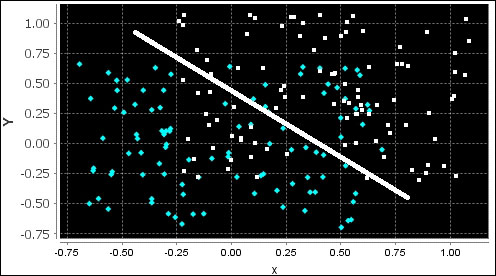
The following chart describes the high margin; the first training set generated with the parameters a = 0.6 and b = 0.3 illustrates the highly separable classes with a clean and distinct hyperplane:

The following chart describes the medium margin; the parameters a = 0.8 and b = 0.3 generate two groups of observations with some overlap:

The following chart describes the low margin; the two groups of observations in this last training are generated with a = 1.4 and b = 0.3 and show a significant overlap:
The test set is generated in a similar fashion as the training set, as they are extracted from the same data source:
val EPS = 0.0001; val C = 1.0; val GAMMA = 0.8
val N = 100; val COEF0 = 0.5; val DEGREE = 2

val a = 1.4; val b = 0.3  //3 sets of values
val trainSet = genData(a, b) ++ genData(a, 1-b)
val testSet = genData(a, b) ++ genData(a, 1-b)
val labels = Array.fill(N)(0.0) ++ Array.fill(N)(1.0)

val result =
  evalKernel(trainSet,testSet, labels, RbfKernel(GAMMA)) ::
  evalKernel(trainSet,testSet, labels, SigmoidKernel(GAMMA)) ::
  evalKernel(trainSet,testSet, labels, LinearKernel) ::
  evalKernel(trainSet,testSet, labels, PolynomialKernel(GAMMA, COEF0, DEGREE)) :: List[Double]()
The value of the kernel function parameters are arbitrary selected from text books. The evalKernel method defined earlier is applied to the three training sets: high margin (a = 1.4), medium margin (a = 0.8), and low margin (a = 0.6) with each of the four kernels (RBF, sigmoid, linear, and polynomial).
The accuracy is assessed by counting the number of observations correctly classified for all of the classes for each invocation of the predictor, |>:

Comparative chart of kernel functions
Although the different kernel functions do not differ in terms of the impact on the accuracy of the classifier, you can observe that the RBF and polynomial kernels produce slightly more accurate results. As expected, the accuracy decreases as the margin decreases. A decreasing margin is a sign that the cases are not easily separable, affecting the accuracy of the classifier:

Note
Test case design
The test to compare the different kernel methods is highly dependent on the distribution or mixture of data in the training and test sets. The synthetic generation of data in this test case is used for the purpose of illustrating the margin between classes of observations. Real-world datasets may produce different results.
In summary, there are four steps in creating a SVC-based model:
- Select a features set.
- Select the C-penalty (inverse regularization).
- Select the kernel function.
- Tune the kernel parameters.
As mentioned earlier, this test case relies on synthetic data to illustrate the concept of margin and compare kernel methods. Let's use the support vector classifier for a real-world financial application.
The purpose of the test case is to evaluate the risk for a company to curtail or eliminate its quarterly or yearly dividend. The features selected are financial metrics relevant to a company's ability to generate cash flow and pay out its dividends over the long term.
We need to select any subset of the following financial technical analysis metrics (refer to the Terminology section in Appendix A, Basic Concepts):
- Relative change in stock prices over the last 12 months
- Long-term debt-equity ratio
- Dividend coverage ratio
- Annual dividend yield
- Operating profit margin
- Short interest (ratio of shares shorted over the float)
- Cash per share-share price ratio
- Earnings per share trend
The earnings trend has the following values:
- -2, if earnings per share decline by more than 15 percent over the last 12 months
- -1, if earnings per share decline between 5 percent and 15 percent
- 0, if earning per share is maintained within 5 percent
- +1, if earnings per share increase between 5 percent and 15 percent
- +2, if earnings per share increase by more than 15 percent
The features are normalized with values 0 and 1.
The labeled output, dividend changes, is categorized as follows:
- -1, if dividend is cut by more than 5 percent
- 0, if dividend is maintained within 5 percent
- +1, if dividend is increased by more than 5 percent
Let's combine two of these three labels {-1, 0, 1} to generate two classes for the binary SVC:
- Class C1 = stable or decreasing dividends and class C2 = increasing dividends; represented by
dividendsA - Class C1 = decreasing dividends and class C2 = stable or increasing dividends; represented by
dividendsB
The different tests are performed with a fixed set of configuration parameters C and GAMMA and a 2-fold validation configuration:
val path = "resources/data/chap8/dividendsA.csv"
val C = 1.0; val GAMMA = 0.5; val EPS = 1e-3; val NFOLDS = 2

val extractor = relPriceChange :: debtToEquity :: dividendCoverage :: cashPerShareToPrice :: epsTrend :: dividendTrend :: List[Array[String] =>Double]()  //1
The components of the extractor are functions that convert a set of fields in the input .csv file into double floating point values:
val xs = DataSource(path, true, false, 1) |> extractor
val config = SVMConfig(new CSVCFormulation(C),
                       RbfKernel(GAMMA),
                       SVMExecution(EPS, NFOLDS))
val features = XTSeries.transpose(xs.take(xs.size-1))//2
val svc = SVM[Double](config, features, xs.last)

svc.accuracy match { //3
  case Some(acc) => Display.show(s"Accuracy: $acc", logger)
  case None => { … }
}
The different fields are extracted from the dividendsA.csv file using the DataSource extractor with a filter (line 1). The purpose of the test A is to create a separating hyperplane (the predictive model) for dividendsA, that is, companies that cut or maintained their dividends and the companies that increased their dividends. The last field in the extractor is the labeled output. The observed features time series is created from all the fields extracted from the .csv file except the last. The time series has to be transposed to use the format required by LIBSVM (line 2). Once the support vector classifier is created, you can retrieve the accuracy of the cross-validation (line 3).
Tip
LIBSVM scaling
LIBSVM supports feature normalization known as scaling, prior to training. The main advantage of scaling is to avoid attributes in greater numeric ranges dominating those in smaller numeric ranges. Another advantage is to avoid numerical difficulties during the calculation. In our examples, we use the normalization of the time series, XTSeries.normalize. Therefore, the scaling flag in LIBSVM is disabled.
The test is repeated with a different set of features and consists of comparing the accuracy of the support vector classifier for different features sets. The features sets are selected from the content of the .csv file by assembling the extractor with different configurations, as follows:
val extractor = … :: dividendTrend :: List[Array[String] =>Double]()

The test demonstrates that the selection of the proper features set is the most critical step in applying the support vector machine, and any other model for that matter, to classification problems. In this particular case, the accuracy is also affected by the small size of the training set. The increase in the number of features also reduces the contribution of each specific feature to the loss function.
The same process is repeated for the test B whose purpose is to classify companies with decreasing dividends and companies with stable or increasing dividends, as shown in the following graph:

The difference in terms of accuracy of prediction between the first three features set and the last two features set in the preceding graph is more pronounced in test A than test B. In both tests, the feature eps (earning per share) trend improves the accuracy of the classification. It is a particularly good predictor for companies with increasing dividends.
The problem of predicting the distribution (or not) dividends can be restated as evaluating the risk of a company to dramatically reduce its dividends.
What about the risk a company entails to eliminate its dividend altogether? Such a scenario is rare, and those cases are actually outliers. A one-class support vector classifier can be used to detect outliers or anomalies [8:13].