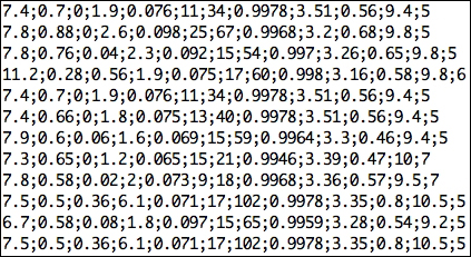
We then import the semicolon-separated text file. We map each line into an Array[String] by splitting each of them using semicolons. We end up with RDD[Array[String]]:

val rdd = sc.textFile("winequality-red.csv").map(line => line.split(";"))

As we discussed earlier, supervised learning requires training data to be provided. We are also are required to test the model that we create for its accuracy against another set of data—the test data. If we have two different datasets for this, we can import them separately and mark them as a training set and a test set. In our example, we'll use a single dataset and split it into training and test sets.

Each of our training samples has the following format: the last field is the quality of the wine, a rating from 1 to 10, and the first 11 fields are the properties of the wine. So, from our perspective, the quality of the wine is the y variable (the output) and the rest of them are x variables (input). Now, let's represent this in a format that Spark understands—a LabeledPoint. A LabeledPoint is a simple wrapper around the input features (our x variables) and our pre-predicted value (y variable) for these x input values:

val dataPoints=rdd.map(row=>new LabeledPoint(row.last.toDouble,Vectors.dense(row.take(row.length-1).map(str=>str.toDouble))))

The first parameter to the constructor of the LabeledPoint is the label (y variable), and the second parameter is a vector of input variables.

As we discussed earlier, we can have two different independent datasets for training and testing. However, it is a common practice to split the dataset into training and test datasets. In this recipe, we will be splitting the dataset into training and test sets in the ratio of 80:20, with each of the elements being selected randomly. This random shuffling of data is one of the prerequisites for better performance of the SGD too:

val dataSplit = dataPoints.randomSplit(Array(0.8, 0.2))
val trainingSet = dataSplit(0)
val testSet = dataSplit(1)

Running a quick summary statistics reveals that our features aren't in the same range:

val featureVector = rdd.map(row => Vectors.dense(row.take(row.length-1).map(str => str.toDouble)))
print(s"Max : ${stats.max}, Min : ${stats.min}, and Mean : ${stats.mean} and Variance : ${stats.variance}")
println ("Min "+ stats.min)
println ("Max "+ stats.max)

Here is the output:

Min [4.6,0.12,0.0,0.9,0.012,1.0,6.0,0.99007,2.74,0.33,8.4]
Max [15.9,1.58,1.0,15.5,0.611,72.0,289.0,1.00369,4.01,2.0,14.9]
Variance : [3.031416388997815,0.0320623776515516,0.03794748313440582,1.987897132985963,0.002215142653300991,109.41488383305895,1082.1023725325845,3.56202945332629E-6,0.02383518054541292,0.02873261612976197,1.135647395000472]

It is always recommended that the input variables have a mean of 0. This is easily achieved with the help of the StandardScaler built into the Spark ML library itself. The one thing that we have to watch out for here is that we have to scale the training and the test sets uniformly. The way we do it is by creating a scaler for trainingSplit and using the same scaler to scale the test set. Another side note is that feature scaling helps with faster convergence in SGD:

val scaler = new StandardScaler(withMean = true, withStd = true).fit(trainingSet.map(dp => dp.features))

val scaledTrainingSet = trainingSet.map(dp => new LabeledPoint(dp.label, scaler.transform(dp.features))).cache()

val scaledTestSet = testSet.map(dp => new LabeledPoint(dp.label, scaler.transform(dp.features))).cache()

The next step is to use our training data to create a model. This just involves creating an instance of LinearRegressionWithSGD and passing in a few parameters: one for the LinearRegression algorithm and two for the SGD. The SGD parameters can be accessed through the use of the optimizer attribute inside LinearRegressionWithSGD:

This step is just a one-liner. We use the resulting model to predict the output (y) based on the features of the test set:

val predictions:RDD[Double]=model.predict(scaledTestSet.map(point=>point.features))

Let's evaluate our model against one of the most popular regression evaluation metrics—mean squared error. Let's get the actual values that our test data has (the y variable prepared manually) and then compare it with the predictions from our model:

val actuals:RDD[Double]=scaledTestSet.map(_.label)

Mean squared error

Note

The mean squared error is given by this formula:

So, we take the difference between the actual and the predicted values (errors), square them, and calculate the sum of them all. We then divide this sum by the number of values, thereby calculating the mean:

val predictsAndActuals: RDD[(Double, Double)] = predictions.zip(actuals)

val sumSquaredErrors=predictsAndActuals.map{case (pred,act)=>
  println (s"act, pred and difference $act, $pred ${act-pred}")
  math.pow(act-pred,2)
}.sum()

val meanSquaredError = sumSquaredErrors / scaledTestSet.count

println(s"SSE is $sumSquaredErrors")
println(s"MSE is $meanSquaredError")

Here is the output:

SSE is 162.21647197365706
MSE is 0.49607483783992984

In our example, we selected all the features that are present in our dataset. Later, we'll take a look at dimensionality reduction, which helps us reduce the number of features while still maintaining the variance of the dataset at a reasonably higher level.

Before we see what regularization is, let's briefly see what overfitting is. A model is said to be overfit (or having high variance) when it memorizes the training set. The result of this is that the algorithm fails to generalize and therefore performs badly with unseen datasets. One way to solve the problem of overfitting is to manually select the important features that will be used to create the model, but for a large-dimensional dataset, it is hard to decide which ones to keep and which ones to throw away.

The other popular option is to retain all the features but reduce the magnitudes of the feature weights. Thus, even with a model that is complex (with higher degree polynomials), if the feature weights are really small, the resulting model would be simple. In other words, given two equally (or almost equally) performing models, with one model being complex (with higher degree polynomial) and the other model being simple, regularization chooses the simple model. The reasoning behind this is that models with simple parameters have a higher probability of predicting unseen data (also known as generalization).

The Spark MLlib comes with implementations for the most common L1 and L2 regularizations. As a side note, LinearRegressionWithSGD, by default, uses a SimpleUpdater, which does not regularize the parameters. Interestingly, Spark has implementations of regression algorithms that are based on top of the L1 and L2 updaters; they are called the Lasso (that uses the L1 updater) and Ridge (that uses the L2 updater by default).

While the L1 regularizer offers some feature selection when the dataset that we have is sparse (or if the dataset's rows are smaller than the feature itself), most of the time, it is recommended is to use the L2 regularizer. The new Pipeline API also has out-of-the-box support for ElasticNet regularization, which uses both the L1 and L2 regularizations internally. Now, let's go over the code:

def algorithm(algo: String, iterations: Int, stepSize: Int) = algo match {
    case "linear" => {
      val algo = new LinearRegressionWithSGD()
algo.setIntercept(true).optimizer.setNumIterations(iterations).setStepSize(stepSize)
      algo
    }
    case "lasso" => {
      val algo = new LassoWithSGD()
algo.setIntercept(true).optimizer.setNumIterations(iterations).setStepSize(stepSize)
      algo
    }
    case "ridge" => {
      val algo = new RidgeRegressionWithSGD()
algo.setIntercept(true).optimizer.setNumIterations(iterations).setStepSize(stepSize)
      algo
    }
  }

As discussed earlier, LassoWithSGD wraps an L1 updater and RidgeRegessionWithSGD wraps an L2 updater. From a code perspective, all that we need to do is change the name of the class. The optimizer (gradient descent) now accepts a regularization parameter that penalizes larger parameters for the features. The default value of the regularization parameter is 0.01 in Spark. A smaller regularization parameter would result in underfitting, and a large parameter would result in overfitting.

The following output shows that regularizing the parameters has reduced our error values:

************** Printing metrics for Linear Regression with SGD *****************
SSE is 132.39124792957116
MSE is 0.4124337941731189
************** Printing metrics for Lasso Regression with SGD *****************
SSE is 132.3943810653321
MSE is 0.4124435547206608
************** Printing metrics for Ridge Regression with SGD *****************
SSE is 132.44011034123344
MSE is 0.4125860135240917

Instead of going through our dataset one by one in the case of SGD, or seeing the entire dataset for every iteration (in the case of batch gradient descent) while updating the parameter vector, we can settle for something in the middle. With the mini batch fraction parameter, for every single iteration, the SGD considers that fraction of the dataset to process for the parameter update. Let's set the batch size to 5 percent:

algo.setIntercept(true).optimizer.setNumIterations(iterations).setStepSize(stepSize).setRegParam(0.001).setMiniBatchFraction(0.05)

The results are as follows:

************** Printing metrics for Linear Regression with SGD *****************
SSE is 112.96958667767147
MSE is 0.3574986920179477
SST is 183.05305027649794
Residual sum of squares is 0.38285875866568087
************** Printing metrics for Lasso Regression with SGD *****************
SSE is 112.95392101963424
MSE is 0.35744911715074124
SST is 183.05305027649794
Residual sum of squares is 0.3829443385454675
************** Printing metrics for Ridge Regression with SGD *****************
SSE is 112.9218089913291
MSE is 0.3573474968080035
SST is 183.05305027649794
Residual sum of squares is 0.3831197632557175

The advantage that we get from using mini batches is that this obviously gives better performance than plain SGD without batches. This is because with plain SGD, for every iteration, only one example is considered to update the parameters. However, with mini batches, we consider a batch of examples. That said, the improvement in the mean squared error from the previous run is not the result of using batches, but just a feature of SGD—roaming around the minima and not converging at a fixed point.