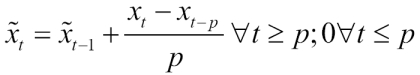
Simple moving average, a smoothing method, is the simplest form of the moving averages algorithms [3:1]. The simple moving average of period p estimates the value at time t by computing the average value of the previous p observations using the following formula:

Note

The simple moving average of a time series {xt} with a period p is computed as the average of the last p observations:

The computation is implemented iteratively using the following formula (1):

Here, is the estimate or simple moving average value at time t.

Let's build a class hierarchy of moving average algorithms, with the abstract parameterized class MovingAverage[T <% Double] as its root. We use the generic time series class, XTSeries[T], introduced in the first section and the generic pipe operator, |>, introduced in the previous chapter:

abstract class MovingAverage[T <% Double] extends PipeOperator[XTSeries[T], XTSeries[Double]]

The pipe operator for the SimpleMovingAverage class implements the iterative formula (1) for the computation of the simple moving average. The override keyword is omitted:

class SimpleMovingAverage[@specialized(Double) T <% Double](val period: Int)(implicit num: Numeric[T]) extends MovingAverage[T] {
   
  def |> : PartialFunction[XTSeries[T], XTSeries[Double]] {
    case xt: XTSeries[T] if(xt != null && xt.size > 0) => {
      val slider = xt.take(data.size-period)
                      .zip(data.drop(period)) //1
      val a0 = xt.take(period).toArray.sum/period //2
      var a: Double = a0
      val z = Array[Array[Double]]( 
       Array.fill(period)(0.0), a, slider.map(x => {
                                     a += (x._2 - x._1)/period
                                     a}) 
    ).flatten //3
    XTSeries[Double](z)
  }

The class is parameterized for the type of elements of the input time series. After all, we do not have control over the source of the input data. The type for the elements of the output time series is Double.

The class has a type T and is specialized for the Double type for faster processing. The implicitly defined num: Numeric[T] is required by the arithmetic operators sum and / (line 2).

The implementation has a few interesting elements. First, the set of observations is duplicated and the index in the clone is shifted by p observations before being zipped with the original to the array of a pair of values: slider (line 1):

The sliding algorithm to compute moving averages

The average value is initialized with the average of the first p data points. The first p values of the trends are initialized as an array of p zero values. It is concatenated with the first average value and the array containing the remaining average values. Finally, the array of three arrays is flattened (flatten) into a single array containing the average values (line 3).

The weighted moving average method is an extension of the simple moving average by computing the weighted average of the last p observations [3:2]. The weights α_j are assigned to each of the last p data points x_j, and are normalized by the sum of the weights.

Note

The weighted moving average of a series {xt} with a period p and a normalized weights distribution {αj} is given by the following formula (2):

Here, is the estimate or simple moving average value at time t.

The implementation of the WeightedMovingAverage class requires the computation of the last p data points. There is no simple iterative formula to compute the weighted moving average at time t+1 using the moving average at time t:

class WeightedMovingAverage[@specialized(Double) T <% Double](val weights: DblVector) extends MovingAverage[T]  {
  def |> : PartialFunction[XTSeries[T], XTSeries[Double]] = {
    case xt: XTSeries[T] if(xt != null && xt.size > 1) => {
     val smoothed =  Range(weights.size, xt.size).map(i => {
        xt.toArray.slice(i- weights.size , i)
                  .zip(weights)
                  .foldLeft(0.0)((s, x) => s + x._1*x._2) }) //1
     XTSeries[Double](Array.fill(weights.size)(0.0) ++ smoothed) //2
   }
}

As with the simple moving average, the array of the initial p moving average with the value 0 is concatenated (line 2) with the first moving average value and the remaining weighted moving average computed using a map (line 1). The period for the weighted moving average is implicitly defined as weights.size.

The exponential moving average is widely used in financial analysis and marketing surveys because it favors the latest values. The older the value, the less impact it has on the moving average value at time t [3:3].

Note

The exponential moving average on a series {xt} and a smoothing factor is computed by the following iterative formula:

Here, is the value of the exponential average at t.

The implementation of the ExpMovingAverage class is rather simple. There are two constructors, one for a user-defined smoothing factor and one for the Nyquist period, p, used to compute the smoothing factor alpha = 2/(p+1):

class ExpMovingAverage[@specialized(Double) T <% Double](val alpha: Double) extends MovingAverage[T]  {
  def |> : PartialFunction[XTSeries[T], XTSeries[Double]] = {
    case xt: XTSeries[T] if(xt != null && xt.size > 1) => {
      val alpha_1 = 1-alpha
      var y: Double = data(0)
      xt.map( x => {
        val z = x*alpha + y*alpha_1; y=z; z })
    }
  }
}

The version of the constructor that uses the Nyquist period p is implemented using the Scala apply method:

def apply[T <% Double](nyquist: Int): ExpMovingAverage[T] = new ExpMovingAverage[T](2/( nyquist + 1))

Let's compare the results generated from these three moving averages methods with the original price. We use a data source (with respect to sink), DataSource (with respect to DataSink) to load the historical daily closing stock price of Bank of America (BAC). The DataSource and DataSink classes are defined in the Data extraction section in Appendix A, Basic Concepts. The comparison of results can be done using the following code:

val p_2 = p >>1
val w = Array.tabulate(p)(n =>if(n==p_2) 1.0 else 1.0/(Math.abs(n-p_2)+1)) //1
val weights = w map { _ / w.sum } //2

val src = DataSource("resources/data/chap3/BAC.csv, false)//3

val price = src |> YahooFinancials.adjClose  //4 
val sMvAve = SimpleMovingAverage(p)  
val wMvAve = WeightedMovingAverage(weights)
val eMvAve = ExpMovingAverage(p)

val results = price :: sMvAve.|>(price) :: wMvAve.|>(price)  ::  eMvAve.|>(price)  :: List[XTSeries[Double]]() //5
Val outFile = "output/chap3/mvaverage" + p.toString + ".csv"
DataSink[Double]( outFile) |> results //6

The coefficients for the weighted moving average are generated (line 1) and normalized (line 2). The trading data regarding the ticker symbol, BAC, is extracted from the Yahoo! finances CSV file (line 3), YahooFinancials, using the adjClose extractor (line 4). The smoothed data generated by each of the moving average techniques are concatenated into a list of time series (line 5). Finally, the content is formatted and dumped into a file, outFile, using a DataSink instance (line 6).

The weighted moving average method relies on a symmetric distribution of normalized weights computed by a function passed as an argument of the generic tabulate method. Note that the original price time series is generated if a specific moving average cannot be computed. The following graph is an example of a symmetric filter for weighted moving averages:

The three moving average techniques are applied to the price of the stock of Bank of America (BAC) over 200 trading days. Both the simple and weighted moving average uses a period of 11 trading days. The exponential moving average method uses a scaling factor of 2/(11+1) = 0.1667.

11-day moving averages of the historical stock price of Bank of America

The three techniques filter the noise out of the original historical price time series. The exponential moving average reacts to a sudden price fluctuation despite the fact that the smoothing factor is low. If you increase the period to 51 trading days or two calendar months, the simple and weighted moving averages generate a smoothed time series compared to the exponential moving average with a smoothing factor of 2/(p+1)= 0.038.

51-day moving averages of the historical stock price of Bank of America

You are invited to experiment further with different smooth factors and weight distributions. You will be able to confirm the following basic rule: as the period of the moving average increases, noise with decreasing frequencies is eliminated. In other words, the window of allowed frequencies is shrinking. The moving average acts as a low-band filter that allows only lower frequencies. Fine-tuning the period or smoothing factor is time consuming. Spectral analysis, or more specifically, Fourier analysis, transforms the time series into a sequence of frequencies, which is a time series in the frequency domain.