A time series {x_k} can be represented as a discrete real-time domain function f, x=f(t). In the 18th century, Jean Baptiste Joseph Fourier demonstrated that any continuous periodic function f could be represented as a linear combination of sine and cosine functions. The discrete Fourier transform (DFT) is a linear transformation that converts a time series into a list of coefficients of a finite combination of complex or real trigonometric functions, ordered by their frequencies.

The frequency ω of each trigonometric function defines one of the harmonics of the signal. The space that represents signal amplitude versus frequency of the signal is known as the frequency domain. The generic DFT transforms a time series into a sequence of frequencies defined as complex numbers ω = a + j.φ (j₂= -1), for which a is the amplitude of the frequency and φ is the phase.

This section is dedicated to the real DFT that converts a time series into an ordered sequence of frequencies with real values.

Note

Real discrete Fourier transform

A periodic function f can be represented as an infinite combination of sine and cosine functions:

The Fourier cosine transform of a function f is defined as:

The discrete real cosine series of a function f(-x) = f(x) is defined as:

The Fourier sine transform of a function is defined as:

The discrete real sine series of a function f(-x) = f(x) is defined as:

The computation of the Fourier trigonometric series is time consuming with an asymptotic time complexity of O(n2). Several attempts have been made to make the computation as effective as possible. The most common numerical algorithm used to compute the Fourier series is the fast Fourier transform created by J. W. Cooley and J. Tukey [3:7]. The algorithm, called Radix-2, recursively breaks down the Fourier transform for a time series of N data points into any combination of N1 and N2 sized segments such as N = N1 N2. Ultimately, the discrete Fourier transform is applied to the deepest-nested segments.

The Radix-2 implementation requires that the number of data points is N=2n for even functions (sine) and N = 2n+1 for cosine. There are two approaches to meet this constraint:

Padding the original time series is the preferred option because it does not affect the original set of observations.

Let's define a base class, DTransform[T], for all the fast Fourier transforms, parameterized with a view bounded to the Double type (Double, Float, and so on). The first step is to implement the padding method, common to all the Fourier transforms:

trait DTransform[T] extends PipeOperator[XTSeries[T], XTSeries[Double]] {
  def padSize(xtSz: Int, even: Boolean=true): Int = {
     val sz = if( even ) xtSz else xtSz-1
     if( (sz & (sz-1)) == 0) 0
     else {
        var bitPos = 0
        do {
        bitPos += 1
        } while( (sz >> bitPos) > 0)
        (if(even) (1<<bitPos) else (1<<bitPos)+1) - xtSz
     }
  }
   
  def pad(xt: XTSeries[T], even: Boolean=true)
           (implicit f: T => Double): DblVector = {
     val newSize = padSize(xt.size, even)
     val arr: DblVector = xt
     if( newSize > 0) arr ++ Array.fill(newSize)(0.0)  else arr
  }
}

The fast implementation of the padding method, pad, consists of detecting the number of observations, N, which is a power of 2 using the bit operator & by evaluating whether N & (N-1) is null. The next highest radix is extracted by computing the number of bits shift in N. The code illustrates the effective use of implicit conversion to make the code readable. The arr: DblVector = series conversion triggers a conversion defined in the XTSeries companion object.

The next step is to write the DFT class for the real discrete transforms, sine and cosine, by subclassing DTransform. The purpose of the class is to select the appropriate Fourier series, pad the time series to the next power of 2 if necessary, and invoke the FastSineTransformer and FastCosineTransformer classes of the Apache Commons Math library [3:8] introduced in the first chapter:

class DFT[@specialized(Double) T<%Double] extends DTransform[T] {
  def |> : PartialFunction[XTSeries[T], XTSeries[Double]] = {
    case xt: XTSeries[T] if(xt != null && xt.length > 0) => 
      XTSeries[Double](fwrd(xt)._2)
  }
  def fwrd(xt:XTSeries[T]): (RealTransformer, DblVector)= {
     val rdt = if(Math.abs(xt.head) < DFT_EPS) 
     new FastSineTransformer(DstNormalization.STANDARD_DST_I)
     else new FastCosineTransformer(DctNormalization.STANDARD_DCT_I)
   
     (rdt, rdt.transform( pad(xt,xt.head==0.0),TransformType.FORWARD))
   }
}

The discrete Fourier sine series requires that the first value of the time series is 0.0. This implementation automates the selection of the appropriate series by evaluating series.head. This example uses the standard formulation of the cosine and sine transformation, defined by the DctNormalization.STANDARD_DCT_I argument. The orthogonal normalization, which normalizes the frequency by a factor of 1/sqrt(2(N-1), where N is the size of the time series, generates a cleaner frequency spectrum for a higher computation cost.

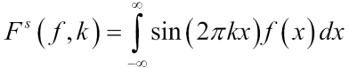
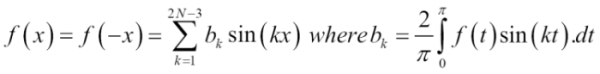
In order to illustrate the different concepts behind DFTs, let's consider the case of a time series generated by a sequence h of sinusoidal functions:

val _T= 1.0/1024
val h = (x:Double) =>2.0*Math.cos(2.0*Math.PI*_T*x) + Math.cos(5.0*Math.PI*_T*x) + Math.cos(15.0*Math.PI*_T*x)/3

As the signal is synthetically created, we can select the size of the time series to avoid padding. The first value in the time series is not null, so the number of observations is 2n+1. The data generated by the function h is plotted as follows:

Example of the sinusoidal time series

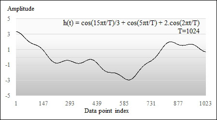
Let's extract the frequencies spectrum for the time series generated by the function h. The data points are created by tabulating the function h. The frequencies spectrum is computed with a simple invocation of the pipe operator on the instance of the DFT class:

val rawOut = "output/chap3/raw.csv"
val smoothedOut = "output/chap3/smoothed.csv"
val values = Array.tabulate(1025)(x =>h(x/1025))
DataSink[Double](rawOut) |> values //1

val smoothed = DFT[Double] |> XTSeries[Double](values) //2
DataSink[Double]("output/chap3/smoothed.csv") |> smoothed

The first data sink (the type DataSink) stores the original time series into a CSV file (line 1). The DFT instance extracts the frequencies spectrum and formats it as time series (line 2). Finally, a second sink saves it into another CSV file.

The spectrum of the time series, plotted for the first 32 points, clearly shows three frequencies at k=2, 5, and 15. This is expected because the original signal is composed of three sinusoidal functions. The amplitude of these frequencies are 1024/1, 1024/2, and 1024/6, respectively. The following plot represents the first 32 harmonics for the time series:

Frequency spectrum for a three-frequency sinusoidal

The next step is to use the frequencies spectrum to create a low-pass filter using DFT. There are many algorithms to implement a low or pass band filter in the time domain from autoregressive models to the Butterworth algorithm. However, the fast Fourier transform is still a very popular technique to smooth signals and extract trends.

The purpose of this section is to introduce, describe, and implement a noise filtering mechanism that leverages the discrete Fourier transform. The idea is quite simple: the forward and inverse Fourier transforms are used sequentially to convert the time series from the time domain to the frequency domain and back. The only input you need to supply is a function G that modifies the sequence of frequencies. This operation is known as the convolution of the filter G and the frequencies spectrum. A convolution is similar to an inner product of two time series in the frequencies domain. Mathematically, the convolution is defined as follows:

Note

Convolution

The convolution of two functions f and g is defined as:

DFT convolution

One important property of the Fourier transform is that convolution of two signals is implemented as the inner product of their relative spectrums:

Let's apply the property to the discrete Fourier transform. If a time series {xⁱ} has a frequency spectrum and a filter f in a frequency domain defined as , then the convolution is defined as:

Let's apply the convolution to our filtering problem. The filtering algorithm using the discrete Fourier transform consists of five steps:

The most commonly used low-pass filters are known as the sinc and sinc2 functions, defined as a rectangular function and a triangular function, respectively. The simplest low-pass filter is implemented by a sinc function that returns 1 for frequencies below a cutoff frequency, fC, and 0 if the frequency is higher:

def sinc(f: Double, fC: Double): Double = if(Math.abs(f) < fC) 1.0 else 0.0
def sinc2(f: Double, fC: Double): Double = if(f*f < fC) 1.0 else 0.0

The filtering computation is implemented as a data transformation (pipe operator |>). The DFTFir class inherits from the DFT class in order to reuse the fwrd forward transform function. As usual, exception and validation code is omitted. The frequency domain function g is an attribute of the filter. The g function takes the frequency cutoff value fC as the second argument. The two filters sinc and sinc2 defined in the previous section are examples of filtering functions.

class DFTFir[T <% Double](val g: (Double, Double) =>Double, val fC; Double) extends DFT[T]

The pipe operator implements the filtering functionality:

def |> : PartialFunction[XTSeries[T], XTSeries[Double]] = {
  case xt: XTSeries[T] if(xt != null && xt.size > 2) => {
    val spectrum = fwrd(xt) //1
    val cutOff = fC*spectrum._2.size
    val filtered = spectrum._2.zipWithIndex.map(x => x._1*g(x._2, cutOff)) //2
    XTSeries[Double](spectrum._1.transform(filtered, TransformType.INVERSE)) //3
}

The filtering process follows three steps:

Let's evaluate the impact of the cutoff values on the filtered data. The implementation of the test program consists of invoking the DFT filter pipe operator and writing results into a CSV file. The code reuses the generation function h introduced in the previous paragraph:

val price = src |> YahooFinancials.adjClose  
val filter = new DFTFir[Double](sinc, 4.0)
val filteredPrice = filter |> price

Filtering out the noise is accomplished by selecting the cutoff value between any of the three harmonics with the respective frequencies of 2, 5, and 15. The original and the two filtered time series are plotted on the following graph:

Plotting of the discrete Fourier filter-based smoothing

As you would expect, the low-pass filter with a cutoff value of 12 removes the noise with the highest frequencies. The filter (with the cutoff value 4) cancels out the second harmonic (low-frequency noise), leaving out only the main trend cycle.

Using the discrete Fourier transform to generate the frequencies spectrum of a periodical time series is easy. However, what about real-world signals such as the time series representing the historical price of a stock?

The purpose of the next exercise is to detect, if any, the long term cycle(s) of the overall stock market by applying the discrete Fourier transform to the quote of the S&P 500 index between January 1, 2009, and December 31, 2013, as illustrated in the following graph:

Historical S&P 500 index prices

The first step is to apply the DFT to extract a spectrum for the S&P 500 historical prices, as shown in the following graph, with the first 32 harmonics:

Frequencies spectrum for historical S&P index

The frequency domain chart highlights some interesting characteristics regarding the S&P 500 historical prices:

A low-pass filter is limited to reduce or cancel out the noise in the raw data. In this case, a passband filter using a range or window of frequencies is appropriate to isolate the frequency or the group of frequencies that characterize a specific cycle. The sinc function introduced in the previous section to implement a low-band filter is modified to enforce the passband within a window, [w1, w2], as follows:

def sinc(f: Double, w: (Double, Double)): Double = if(Math.abs(f) > w._1 && Math.abs(f) < w._2) 1.0 else 0.0

Let's define a DFT-based pass-band filter with a window of width 4, w=(i, i +4), with i ranging between 2 and 20. Applying the window [4, 8] isolates the impact of the second harmonic on the price curve. As we eliminate the main upward trend with frequencies less than 4, all filtered data varies within a short range relative to the main trend. The following graph shows output of this filter:

The output of a pass-band DFT filter range 4-8 on the historical S&P index

In this case, we filter the S&P 500 index around the third group of harmonics with frequencies ranging from 18 to 22; the signal is converted into a familiar sinusoidal function, as shown here:

The output of a pass-band DFT filter range 18-22 on the historical S&P index

There is a possible rational explanation for the shape of the S&P 500 data filtered by a passband with a frequency of 20, as illustrated in the previous plot; the S&P 500 historical data plot shows that the frequency of the fluctuation in the middle of the uptrend (trading sessions 620 to 770) increases significantly. This phenomenon can be explained by the fact that the S&P 500 index reaches a resistance level around the trading session 545 when the existing uptrend breaks. A tug-of-war starts between the bulls, betting the market nudges higher, and the bears, who are expecting a correction. The back and forth between the traders ends when the S&P 500 index breaks through its resistance and resumes a strong uptrend characterized by a high amplitude and low frequency, as shown in the following graph:

One of the limitations of using the Fourier transform to clean up data is that it requires the data scientist to extract the frequencies spectrum and modify the filter on a regular basis, as he or she is never sure that the most recent batch of data does not introduce noise with a different frequency. The Kalman filter addresses this limitation.