
A support vector machine (SVM) is a linear discriminative classifier that attempts to maximize the margin between classes during training. This approach is similar to the definition of a hyperplane through the training of the logistic regression (refer to the Binomial classification section of Chapter 6, Regularization and Regression). The main difference is that the support vector machine computes the optimum separating hyperplane between groups or classes of observations. The hyperplane is indeed the equation that represents the model generated through training.
The quality of the SVM depends on the distance, known as margin, between the different classes of observations. The accuracy of the classifier increases as the margin increases.
First, let's apply the support vector machine to extract a linear model (classifier or regression) for a labeled set of observations. There are two scenarios for defining a linear model. The labeled observations are as follows:
- Naturally segregated in the features space (the separable case)
- Intermingled with overlap (the nonseparable case)
It is easy to understand the concept of an optimal separating hyperplane in cases the observations are naturally segregated.
The concept of separating a training set of observations with a hyperplane is better explained with a 2-dimensional (x, y) set of observations with two classes, C1 and C2. The label y has the value -1 or +1.
The equation for the separating hyperplane is defined by the linear equation, y=w.xT+w0, which sits in the midpoint between the boundary data points for class C1 (H1: w.xT + w0 + 1=0) and class C2 (H2: w.xT + w0 - 1). The planes H1 and H2 are the support vectors:

Support vector machine – separable case
In the separable case, the support vectors fully segregate the observations into two distinct classes. The margin between the two support vectors is the same for all the observations and is known as the hard margin.
In the nonseparable case, the support vectors cannot completely segregate observations through training. They merely become linear functions that penalize the few observations or outliers that are located outside (or beyond) their respective support vector, H1 or H2. The penalty variable ξ, also known as the slack variable, increases if the outlier is further away from the support vector:

A support vector machine – the nonseparable case
The observations that belong to the appropriate (or own) class do not have to be penalized. The condition is similar to the hard margin, which means that the slack ξ is null. Observations that belong to the class but located beyond its support vector are penalized; the slack ξ increases as the observations get closer to the support vector of the other class and beyond. The margin is then known as a soft margin because the separating hyperplane is enforced through a slack variable.

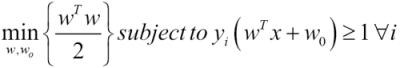
You may wonder how the minimization of the margin error is related to the loss function and the penalization factor introduced for the ridge regression (refer to the Numerical optimization section of Chapter 6, Regularization and Regression). The second factor in the formula corresponds to the ubiquitous loss function. You will certainly recognize the first term as the L2 regularization penalty with λ=1/2C.
The problem can be reformulated as the minimization of a function known as the primal problem [8:6].

The C penalty factor can be thought of as the inverse of the L2 regularization factor. The loss function L is then known as the hinge loss. The formulation of the margin using the C penalty (or cost) parameter is known as the C-SVM formulation. C-SVM is sometimes called the C-Epsilon SVM formulation for the nonseparable case.
The υ-SVM (or Nu-SVM) is an alternative formulation to the C-SVM. The formulation is more descriptive than C-SVM; υ represents the upper bound of the training observations that are poorly classified and the lower bound of the observations on the support vectors [8:7].

The C-SVM formulation is used throughout the chapters for the binary, one class support vector classifier as well as the support vector regression.
Note
Sequential Minimal Optimization
The optimization problem consists of the minimization of a quadratic objective function (w2) subject to N linear constraints, N being the number of observations. The time complexity of the algorithm is O(N3). A more efficient algorithm, known as Sequential Minimal Optimization (SMO) has been introduced to reduce the time complexity to O(N2).
So far, it has been assumed that the separating hyperplane, and therefore, the support vectors, are linear functions. Unfortunately, such assumptions are not always correct in the real world.
Support vector machines are known as large or maximum margin classifiers. The objective is to maximize the margin between the support vectors with hard constraints for separable (similarly, soft constraints with slack variables for nonseparable) cases.
The model parameters {wi} are rescaled during optimization to guarantee that the margin is at least 1. Such algorithms are known as maximum (or large) margin classifiers.
The problem of fitting a nonlinear model into the labeled observations using support vectors is not an easy task. A better alternative consists of mapping the problem to a new, higher dimensional space using a nonlinear transformation. The nonlinear separating hyperplane becomes a linear plane in the new space, as illustrated in the following diagram:

Illustration of the Kernel trick in an SVM
The nonlinear SVM is implemented using a basis function, ϕ(x). The formulation of the nonlinear C-SVM is very similar to the linear case. The only difference is the constraint along the support vector, using the basis function, φ:
The minimization of wT.ϕ(x) in the preceding equation requires the computation of the inner product ϕ(x)T.ϕ(x). The inner product of the basis functions is implemented using one of the kernel functions introduced in the first section. The optimization of the preceding convex problem computes the optimal hyperplane w* as the kernelized linear combination of the training samples, y.ϕ(x), and Lagrange multipliers. This formulation of the optimization problem is known as the SVM dual problem. The description of the dual problem is mentioned as a reference and is well beyond the scope of this book [8:8 ].


The transformation (x,x') => K(x,x') maps a nonlinear problem into a linear problem in a higher dimensional space. It is known as the kernel trick.
Let's consider, for example, the polynomial kernel defined in the first section with a degree d=2 and coefficient of C0=1 in a two-dimension space. The polynomial kernel function on two vectors, x=[x1, x2] and z=[x'1, x'2], is decomposed into a linear function in a dimension 6 space:
