The Rug Plot

The rug is not really a separate plot. It is a one-dimensional display that you can add to existing plots to illuminate information that is sometimes lost in other types of graphs. Like a strip plot, it represents values of a variable by putting a symbol at various points along an axis. However, it uses short lines to represent points. You can place it at the bottom (the default) or top of a graph (side = 3). If appropriate—for example, if a box plot is vertical—the rug can be put on the left (side = 2) or right (side = 4) axis. When two observations have the same value, they are overprinted, so that the line is darker. Here are some examples:

# Script for Figure 11-1
library(multcomp)
par(mfrow = c(2,2))
stripchart(mtcars$drat,
  main="a. side = 3", method = "jitter",
  pch = 20, col = "sienna4")
rug(mtcars$drat, side = 3)

boxplot(mtcars$drat, main = "b. side = 2",
  col = "firebrick")
rug(mtcars$drat, col = "darkmagenta", side = 2)

hist(airquality$Ozone, main = "c. side = 1", col = "cyan4")
rug(airquality$Ozone, col = "cyan4")




boxplot(sbp$sbp,
  main = "d. side = 4", col = "darkorange3")
rug(sbp$sbp, side = 4, col = "cornsilk4")

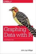
The preceding script produces the plots in Figure 11-1.

Figure 11-1. Uses of the rug plot.

Figure 11-1a shows that adding a rug is essentially like putting a strip chart at the bottom or top of another graph. This is not very useful on strip charts, because the rug is simply redundant. However, the rug can be helpful on other types of graphs to reveal information that might be lost in those displays. For example, in Figure 11-1b, the box plot shows a skewed distribution, but we could not possibly know from the box plot alone that the data is in several clumps, which is clearly shown in the rug. The long upper whisker, for example, might be the result of several dispersed points or simply one extreme value. The rug shows all the points and their placement, with one extreme value and a few points clumped just above the third quartile. Compare that to Figure 11-1d, in which the rug is nearly equally spaced throughout its range. The rug in Figure 11-1c again shows the data to be in clumps. This suggests that changing the bin size can change the shape of the histogram. By default, the rug is placed at the bottom of the graph, but you can place it at the top with the argument side = 3. For more information on the arguments that you can use, type ?rug. The rug can sometimes be very helpful, but at other times it offers no real advantage.

Exercise 11-1

Add a rug plot to a density plot of time from the Nimrod dataset. Add a rug to a box plot of MathAchieve$SES (refer to Figure 5-2). Which of these is more helpful?