Density Estimation

A common problem in science is to estimate, from a data sample, a mathematical function that describes the relative likelihood that a variable (such as the systolic blood pressure in the sbp example in the previous two chapters) takes a particular value. We tried to make a rough estimate of such a graph with histograms in Chapter 7. So, for instance, if you take a glance at the histogram in Figure 7-2, you can see that systolic blood pressures close to 150 are very likely to occur, but scores of about 110 are relatively unlikely. The rule, or formula, that gives the likelihood of a given value of, for example, blood pressure is called the density function.

Histograms are a good tool for many problems, being easy to understand and relatively easy to compute. There is, however, a shortcoming of which you should be aware. Many functions of interest are continuous; that is, they can take any value within a certain range. A blood pressure value could be 120 or 123 or 129.2, yet the histogram might force all of those values to be in the same bin and thereby all to take the value of 120. (Remember that the bin width in the histogram in Figure 7-2 was 10, so all scores equal to or greater than 120 and less than 130 fall within the same bin.) That is to say, we used a discrete function—one  that can only take selected values of blood pressure—to estimate the density function, which is continuous. The graph in Figure 8-1a, a kernel density plot, is a smooth line approximation of the density function.

Figure 8-1. Kernel density of blood pressures and kernel density imposed on a histogram of blood pressures.

Look at the graph in Figure 8-1b to see the density estimate produced by R’s density() function superimposed on the histogram.   You can see that the density curve sometimes goes above the histogram and sometimes below. Imagine that you took several weighted averages of numeric values of groups of adjacent bins and replaced the histogram values with smooth lines connecting those averages. This is a type of smoothing. Several examples appear in Figure 8-1, the script for which is presented here:

# Script for Figure 8-1; there are 4 graphs
library(multcomp)
par(mfrow = c(2,2), cex.main =.9)

# Figure 8-1a
eq = density(sbp$sbp) # estimate density curve of sbp
plot(eq, xlim = c(100,190),
  main = "a. Systolic Blood Pressure Density Plot",
  lwd = 2) # plot estimate

# Figure 8-1b
# use histogram to estimate density
hist (sbp$sbp,
  main = "b. Histogram + Kernel Density", col = "maroon",
  las = 1, cex.axis = .8, freq = F) # freq=F: prob. densities
lines(eq,lwd = 2) # plot density curve on existing histogram

# Figure 8-1c
eq2 = density(sbp$sbp, bw = 5)
hist (sbp$sbp,
  main = "c. Histogram + Kernel Density, bw = 5",
  col = "maroon", las = 1, cex.axis = .8,
  freq = F) # freq=F: prob. densities
lines(eq2,lwd = 2) # plot density curve on existing histogram

# Figure 8-1d
eq3 = density(sbp$sbp, bw = 10)
hist (sbp$sbp,
  main = "d. Histogram + Kernel Density, bw = 10",
  col = "maroon", las = 1,
  cex.axis = .8, freq = F) # freq=F: prob. densities
lines(eq3, lwd = 2) # plot density curve on existing histogram

Figure 8-1a is a kernel density plot. The term kernel refers to the method used to estimate the points that make up the plot. In Figure 8-1b, a new plot is superimposed on top of the existing histogram by using the lines() command. Combining two graphs this way is very useful, and we will use variations of this trick often. In this case, we view two different methods of summarizing a single distribution.

The plot in Figure 8-1a shows the default label on the x-axis, which gives the sample size, N, and the bandwidth. The bandwidth indicates how spread out the plot is. Figures 8-1b, 8-1c, and 8-1d show the effects of changing the bandwidth. Figure 8-1b shows the default bandwidth, the same as Figure 8-1a. Note that it conforms to the general shape of the histogram. It changes direction three times—that is, there are three (very small) bends in the line—and we may well conclude that it is a reasonably good fit to the histogram. Figure 8-1c shows a smaller bandwidth, which fits more tightly to the histogram and changes direction five times. Figure 8-1d shows a larger bandwidth, which results in a flatter line that bends only once.

Comparing Two or More Density Plots

It is sometimes desirable to compare two or more density plots. For example, you might want to compare the means of two distributions and see if they have similar shape and variance. Consider the emissions data from Chapter 1, in the section “Using the Data Editor”:

 

> load("emiss.rda") # load emissions data from Chapter 1
> emissions  # look at emissions data

  Year  N_Amer CS_Amer Europe Eurasia Mid_East Africa 
1 2004   16.2     2.4    7.9     8.5      7.1    1.1
2 2005   16.2     2.5    7.9     8.5      7.6    1.2   
3 2006   15.9     2.5    7.9     8.7      7.7    1.1 
4 2007   15.9     2.6    7.8     8.6      7.6    1.1
5 2008   15.4     2.6    7.7     8.9      7.9    1.2 
6 2009   14.2     2.6    7.1     8.0      8.3    1.1 
7 2010   14.5     2.7    7.2     8.4      8.4    1.1
 Asia_Oceania
1      2.7
2      2.9
3      3.1
4      3.2
5      3.3
6      3.5
7      3.6

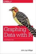
Suppose that we wanted to compare the emission profiles of Europe and Eurasia. We could first make a density plot of the European emissions data and then use the lines() function to plot the Eurasian data on top of it. Notice that the following code for Figure 8-2 makes use of the xlim and ylim arguments.  This is a way of forcing the plot of the European density to be big enough that the plot of the Eurasian density does not run off the graph. Do not be overly impressed by my seemingly awesome foresight here—I tried it first without extending the limits of the graph and made a mess! Sometimes trial and error is the only path to enlightenment. The script to produce the figure follows:

# Script for Figure 8-2
# following par() sets white characters on black background
load("emiss.rda")
par(bg = "black", col.lab = "white",
  col.axis = "white", bty="l",
  fg = "white", col.main = "white")
euro = density(emissions$Europe) # points on density(Euro)
ea = density(emissions$Eurasia)  # points on density(Eurasia)

# use xlim & ylim so 2nd plot does not go out of range
plot(euro, xlim = c(6.9,9), ylim = c(0,2),
  main = "CO2 Emissions in Europe and Eurasia",
  col = "goldenrod1", lwd = 2)
lines(ea, xlim = c(6.9,9), ylim = c(0,2),
  lty = 2, lwd = 2, col = "cyan")
# lty=2 is dotted line  
# lwd = 2 is a wider line than default line

legend("topleft",c("Europe","Eurasia"),
  text.col = c("goldenrod3","cyan"), bty = "n")

Figure 8-2 illustrates what the preceding code produces.

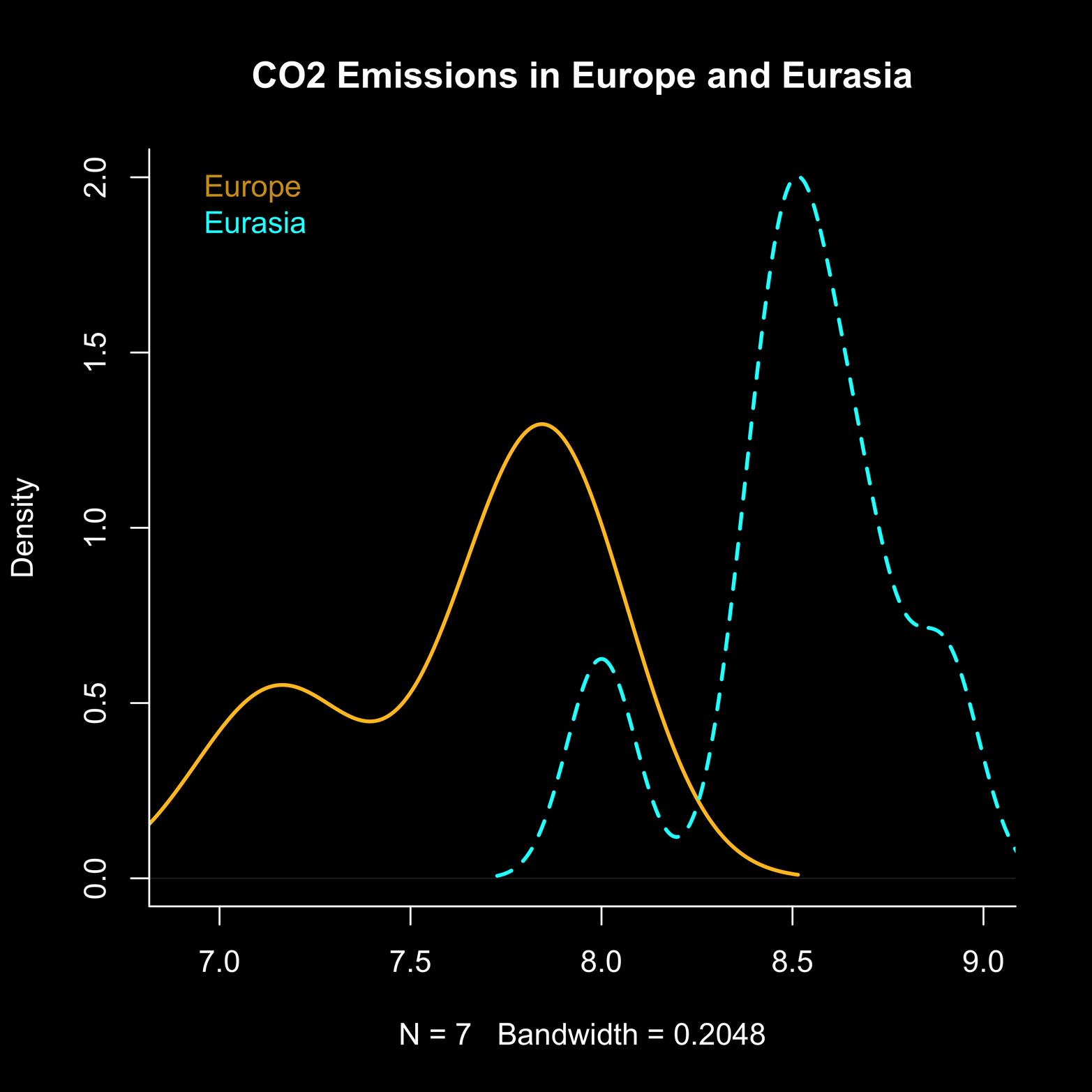
Figure 8-2. Two density plots on the same axis. The xlim and ylim arguments were used in the first plot to make the plotting area big enough to include the second plot, which otherwise would have gone out of range.

The Cumulative Distribution Function

As enlightening as density plots can be, they do not always give us the information we really need. Even though the density plot gives a sense of the relative likelihood of a value on the horizontal axis, oftentimes we would like to know the likelihood of, for example, a systolic blood pressure of 120 or less, or 135 or greater, or between 120 and 140. A plot of the cumulative distribution function (CDF) displays on the y-axis the probability of a score equal to or less than the value on the x-axis.

Consider a data distribution that follows the normal distribution—the so-called “bell curve.” Our example comes from a simulation, or a computer imitation of selecting a large sample of numbers from a population of numbers with specified characteristics. The following code for Figure 8-3 shows how to do this with the rnorm() function:

# code for Figure 8-3
library(multcomp)
library(Hmisc)
par(mfrow = c(2,2), cex.main = .9, bg = "white")

# get 100,000 numbers sampled from a normal dist
# with mean = 0 and sd = 1
sam <- (rnorm(100000))  #mean = 0 and sd = 1 are default values
plot(density(sam),
  main = "a. Density (sampling from Normal distribution)",
  col = "coral4")  # Figure 8-3a
polygon(density(sam), col = "coral4") # color area under curve

plot(ecdf(sam),
  main = "b. Cumulative distribution function of sample in 
  Figure 8-3a", col = "turquoise")

plot(ecdf(sbp$sbp), main = "c. ecdf(sbp$sbp) - base R")


Ecdf(sbp$sbp,
  main="d. Ecdf(sbp$sbp) - Hmisc pack. + grid()",
  xlab = "sys blood pressure", col = "deepskyblue3")
grid(col = "gray70") # adds gray grid to current plot

Figure 8-3. The empirical cumulative distribution function.

The graph in Figure 8-3a is the density plot of the sample of 100,000 numbers generated by the computer. Figure 8-3b shows the CDF of the dataset. You can see from this plot that about half of all the numbers on the y-axis are less than or equal to the x value of 0. You can also easily see that nearly (but not quite) all of the numbers are less than 2. The CDF plot in Figure 8-3b was produced by using R’s ecdf() function, which plots the empirical cumulative density function. It is a smooth curve because there are so many numbers and the distribution is continuous. Figure 8-3c shows what happens when the ecdf() function is applied to the small sbp dataset. The “curve” is interpreted in the same way as it was in Figure 8-3b, but the data is so sparse that there are breaks in the plot, making it less attractive and more difficult to read. Practice reading Figure 8-3c. What blood pressure is greater than about half of all the blood pressures? Find the place on the y-axis equal to proportion = 0.5. The x coordinate is about 150, or slightly less, so about 50 percent of the blood pressures are equal to or less than 150.

An alternative method to find the CDF is to use the Ecdf() function in the Hmisc package. You can see the plot produced by this function in Figure 8-3d. It is a step function rather than a smooth curve, but it is more appealing than the graph in Figure 8-3c, and easier to read. There are many advanced features available with this function, such as the ability to produce graphs for multiple groups and some labeling options. Although there are still other options for producing CDFs, one that is especially interesting is the stat_ecdf() function in the ggplot2 package. Figure 8-4 shows a graph produced by this function. It is both attractive and easy to read, largely because of the grid lines. Following is the code to produce it:

# code for Figure 8-4
library(ggplot2)
ggplot(sbp, aes(x=sbp)) + stat_ecdf()

Figure 8-4. Empirical cumulative density plot produced by the ggplot2 package. The grid lines make this graph relatively easy to read.