Basic Stem-and-Leaf Plot

This short chapter might be considered “nostalgia” by some because it describes a type of graph that was important in the paper-and-pencil days of data analysis. You probably will not see many examples of this type of graph in modern presentations, but it is included here because it will help you to understand the histogram a little better, which is the topic of Chapter 7. You might also find it useful in the exploratory phase of your data examination. If you are already knowledgeable about histograms, you can skip this chapter without fear of missing necessary material.

The sbp dataset in the multcomp package  includes the variables sbp—the systolic blood pressure of 69 patients—and the gender of each of those people as well as the age of each. We can look at the distribution of the blood pressures with a stem-and-leaf plot. This type of graph reveals not only the general shape of the data distribution, but the (rounded) value of each data point as well.

The stem-and-leaf plot works by putting all of the values in order, from lowest to highest. Then, it reserves a line for all of the values in a common range and writes the last significant digit of each number on the appropriate line. You can use the stem() command  in base R to create a stem-and-leaf plot of the sbp variable in the sbp dataset.  This type  of display, sometimes called a textual display, appears in the R console, not in a graphic window. We can produce the display shown in Figure 6-1 as follows:

> library(multcomp)
> stem(sbp$sbp)

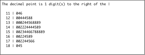
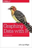
Figure 6-1. A stem-and-leaf plot of the sbp variable

The display in Figure 6-1 shows all the blood pressures in the dataset. The column on the left side of the display, including the numbers 11, 12, 13, and so on, contains the “stems.” The blood pressures are all three-digit numbers, so the stem contains the first two digits, and the “leaf” contains the last digit of each number. Reading from the top of the display, the numbers represented in the first stem are numbers beginning with “11” and the leaves are 0, 4, and 6. Thus, the numbers represented on the first line are 110, 114, and 116. The next stem includes the numbers 120, 120, 124, 124, 124, 125, 128, and 128. We can see that there are exactly two systolic blood pressures of 170 and four of 158, but only one of 185.

Figure 6-1 shows the distribution of the data to be approximately symmetrical. There are about the same number of low blood pressures as there are high blood pressures, and a relatively large number of blood pressures near the center of the distribution (i.e., blood pressures of about 130 to 160). In this figure, the width of a stem is about 10 (e.g., 110–119, 120–129). If the width of the stem is changed, the shape of the graph may well change, too. You can make such a change to the stem width by adding another argument to the stem() command. The argument scale = x, where x is a positive number, controls how wide each stem will be. For example, try this command:

> stem(sbp$sbp, scale = 2)

In Figure 6-2, the graph is twice as long as before. Each stem is half as wide (i.e., width 5 instead of 10), but there are twice as many stems. The general shape of the distribution has not changed very much, although there is a dip in the center, around 145, that we did not see earlier. In some distributions, a change of scale will dramatically change the shape. The width of leaves corresponds to the size of what we will call bins in the histogram. Perhaps the stem-and-leaf plot does not look as appealing as some other types of graph, with nicely formed rectangles and colors. However, this type of plot shows the precise value of each number in the vector studied. This can aid in understanding the data and suggest modifications to make in a graph.

/>

Figure 6-2. Stem-and-leaf plot of sbp, with twice as many stems.

The stem-and-leaf plot works best for small to medium-sized datasets. If there are too many numbers in one stem, they will run off the page! When this happens, we lose all sense of the real shape of the distribution. One way to deal with this is to make the scale bigger. This makes more leaves with fewer numbers in each one of them. Sometimes, even this strategy will not help enough. Again, you might not use this type of plot in a final presentation, but perhaps you will find this elegant tool helpful to understand the histogram and revealing during the exploratory phase of your project.

Exercise 6-1

Try your hand at picking a suitable scale for the blood pressure data. The numbers you choose do not need to be integers. They can also be smaller than 1. Try the same thing with some of the datasets we have examined in earlier chapters.