Chapter 11. Tuning Mule

This chapter covers

• Identifying performance bottlenecks
• Staged event-driven architectures
• Configuring processing strategies

Whether you have predetermined performance goals and want to be sure to reach them or you’ve experienced issues with your existing configuration and want to solve them, the question of tuning Mule will occur to you sooner or later in the lifetime of your projects. Indeed, Mule, like any middleware application, is constrained by the limits of memory size, CPU performance, storage, and network throughput. Tuning Mule is about finding the sweet spot in which your business needs meet the reality of software and hardware constraints.

The same way a race car needs tuning to adapt to the altitude of the track or to the weather it will race in, Mule can require configuration changes to deliver its best performance in the particular context of your project. Up to this point in the book, we’ve relied on the default configuration of Mule’s internal thread pools and haven’t questioned the performance of the different moving parts, whether they’re standard or custom. We’ll now tackle these tough questions.

In short, the objective of this chapter is twofold: to give you a deep understanding of Mule’s threading model and to offer you some hints on how to configure Mule so it reaches your performance targets. This chapter will often make references to previous chapters, as the quest for performance isn’t an isolated endeavor but the outcome of scattered but related activities.

Let’s start by looking deeper into the architecture of Mule than ever before in order to learn how threading works behind the scenes.

11.1. Staged event-driven architecture

An understanding of how Mule processes messages is critical in order to tune Mule applications effectively. Mule flows will use one or more pools of threads to process every message. This architecture, in which an application’s event-processing pipeline is decomposed into processing stages, is one of the core concepts behind a staged event-driven architecture, or SEDA (see figure 11.1). SEDA, as described in Matt Welsh’s paper “SEDA: An Architecture for Highly Concurrent Server Applications,”^[1] is summarized as follows:

¹ See SEDA, Matt Welsh, at www.eecs.harvard.edu/~mdw/proj/seda.

Figure 11.1. A typical staged event-driven architecture (SEDA) implementation

SEDA is an acronym for staged event-driven architecture, and decomposes a complex, event-driven application into a set of stages connected by queues. This design avoids the high overhead associated with thread-based concurrency models, and decouples event and thread scheduling from application logic. By performing admission control on each event queue, the service can be well-conditioned to load, preventing resources from being overcommitted when demand exceeds service capacity. SEDA employs dynamic control to automatically tune runtime parameters (such as the scheduling parameters of each stage), as well as to manage load, for example, by performing adaptive load shedding. Decomposing services into a set of stages also enables modularity and code reuse, as well as the development of debugging tools for complex event-driven applications.

Staged event-driven architectures use event queues to split up an application’s processing stages. Each processing stage uses a thread pool to consume messages of a work queue, eliminating the need to spawn a thread for every request the application needs to process. Because a single thread is no longer handling every request, it becomes more difficult to exhaust the application’s ability to spawn threads. It also ensures that other stages of the processing pipeline aren’t starved of the ability to spawn threads.

In this chapter, you’ll see how processing strategies and exchange patterns dictate how much a given flow can take advantage of Mule’s SEDA underpinnings. Assuming your application is tuned properly, you’ll be able to take full advantage of two important benefits of this architecture. The first, which is made clear in Matt’s paper, is the graceful degradation of your application under load—both expected and contrived (that is, through a denial-of-service attack). The second, and perhaps more important, benefit is that your application will make better use of the available cores on the system it’s running on. The techniques introduced in this chapter will aid you in taking advantage of the latter to ensure you’re making the most use of the cores available to your application.

11.1.1. Roll your own SEDA

Most of the tuning you’ll see in this chapter occurs at the flow level of granularity. You’ll see how Mule’s various tuning knobs allow you to define how a flow receives, processes, and dispatches messages. It’s advisable, however, to consider the concepts of SEDA and how they might apply to your application as a whole.

Mule’s VM transport, discussed in chapter 3, is an excellent mechanism to help break your flows into smaller, composite flows that are decoupled with in-memory queueing. This allows you to realize the benefits of SEDA at the macro level, breaking your application into smaller flows that can be individually tuned and are decoupled with VM queueing.

Reliability patterns and SEDA

In chapter 7, you saw how the VM transport can be used to implement reliability patterns. The technique discussed here is an extension of that approach.

The following example illustrates a simple flow that Prancing Donkey is using to process reporting data. The processing stages include three Java components.

Listing 11.1. Report processing in a single flow

Each component is doing a bunch of nontrivial processing for each message received by the flow, whose payload is a large XML report. In order to maximize throughput, refactor the flow using the VM transport. You’ll break this flow out into three different flows that each use a VM queue to decouple each processing stage.

Listing 11.2. Report processing in three flows

Now that the flow has been decomposed into three discrete flows, you have the ability to tune each individually. You also buy yourself some resiliency if any of these flows becomes a bottleneck. Processing is still able to happen in the other two flows. You could also introduce transactions between the flows, facilitating the reliability patterns discussed in chapter 7.

Concurrency, SEDA, and Mule applications

Make sure any component code you’re using with Mule is thread-safe. Mule applications, particularly fully asynchronous ones, almost guarantee that multiple threads of execution will be running through your components under load. If you know your code isn’t thread-safe, consider using a pool of component objects rather than a singleton.

Now let’s take a look at how you can tune the thread pools used in Mule’s SEDA implementation.

11.2. Understanding thread pools and processing strategies

Mule is designed with various thread pools at its heart. Each thread pool handles a specific task, such as receiving or dispatching messages or invoking message processors in a flow. When a thread is done with a particular task, it hands it off to a thread in the next thread pool before coming back to its own pool. This naturally implies some context switching overhead and hence an impact on performance.

Processing strategies dictate how a message is passed off between these pools. The processing strategy is determined by the exchange-pattern of the endpoints in a flow, whether or not the flow is transactional or the processingStrategy attribute on the flow is configured.

Warning

Don’t mix up your thread pools! The upcoming figures and discussions will help you tell them apart.

Let’s start by digging into the different thread pools that exist in Mule. Figure 11.2 represents the three thread pools that can be involved when a flow handles a message event. It also represents the component pool that may or may not have been configured for any components in the flow (see the discussion in section 6.1.5).

Figure 11.2. Mule relies on three thread pools to handle message events before, inside of, and after each flow.

Understanding the thread pool figures

In the coming figures, pay attention to the thread pool box. If it’s full (three arrows represented), that means that no thread from this pool is under use. If a thread is used, its arrow is filled in (black) and moved out of the thread pool box into the stage in which it’s used. If the thread spans stages, its arrow is stretched accordingly.

The receiver and dispatcher thread pools belong to a particular connector object, whereas the flow thread pool is specific to the flow. This is illustrated in figure 11.3. A corollary of this fact is that if you want to segregate receiver and dispatcher pools for certain flows, you have to configure several connectors.

Figure 11.3. Two flows using the same connector share the same receiver and dispatcher thread pools.

If you “zoom” in on a thread pool, you discover that there’s a buffer alongside the threads themselves, as represented in figure 11.4. Each thread pool is associated with a buffer that can queue pending requests in case no thread is available for processing the message right away. It’s only when this buffer is full that the thread pool itself is considered exhausted. When this happens, Mule will react differently depending on your configuration; it can, for example, reject the latest or oldest request. You’ll see more options in section 11.2.3.

Figure 11.4. Each thread pool has a dedicated buffer that can accumulate pending requests if no thread is available to process the message.

You now have a better understanding of the overall design of the Mule threading model. Next, we’ll look at how the synchronicity of a message event impacts the way thread pools are used.

11.2.1. Processing strategies and synchronicity

At each stage of message event processing, Mule decides if it needs to borrow a thread from the corresponding pool or not. A thread is borrowed from the receiver or the dispatcher pool only if this stage is set to be asynchronous. By extension, the flow thread pool is used only if the message source’s exchange-pattern is one-way. There are several factors that determine if the receiver or the dispatcher will be synchronous or not:

• Configured exchange pattern— If you’ve set an inbound or outbound endpoint’s exchange pattern to be request-response, the receiver or dispatcher will be request-response, respectively.
• Incoming event— If the received message event is synchronous, a receiver can act synchronously even if its inbound endpoint is configured to be one-way.
• Outbound message processor— The final message processor can enforce the dispatching stage to be synchronous.
• Transaction— If the flow is transactional, its receiver and dispatcher will be synchronous no matter how the endpoints are configured.

If you look at figure 11.5, you’ll notice that when both the receiver and the dispatcher have one-way exchange patterns, a thread is borrowed from each pool at each stage of the message processing. This configuration fully uses the SEDA design and therefore must be preferred for flows that handle heavy traffic or traffic subject to peaks. This configuration can’t be used if a client is expecting a response from the flow. Table 11.1 summarizes the pros and cons of this configuration model.

Figure 11.5. In fully asynchronous mode, a thread is borrowed from each pool at each stage of the message processing.

Table 11.1. Pros and cons of fully asynchronous mode

Pros	Cons
Uses SEDA model with three fully decoupled stages	Flow can’t return a response to the caller
Highly performant	Complicates integration with clients that need a response

When a flow needs to return a response to the caller, its message source is configured to be request-response. It’s still possible to use the dispatcher thread pool by configuring the exchange-pattern on the outbound endpoint to be one-way. The threading model of this configuration is shown in figure 11.6. Notice how the receiver thread is used for calling the message processors in the flow; this makes sense when you consider that the last processor in the flow will return the result to the caller on that thread. Table 11.2 presents the pros and cons of this approach.

Figure 11.6. If only the receiver is synchronous, one thread from its pool will be used up to the component method invocation stage.

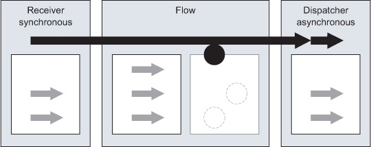
Table 11.2. Pros and cons of the synchronous-asynchronous mode

Pros	Cons
Returns the component response to the caller Dispatching decoupled from receiving and servicing	Receiver thread pool can still be overwhelmed by incoming requests

As discussed in the introduction, a transactional flow will automatically have its receiver and dispatcher running synchronously. Transactions, as you saw in chapter 9, guarantee that message processing in a flow happens in the correct order. To ensure this, transaction processing needs to occur in the same thread. Figure 11.7 demonstrates how the thread used in the receiver is piggybacked all along the processing path of the message event. The pros and cons of this configuration are listed in table 11.3.

Figure 11.7. In fully synchronous mode, the receiver thread is used throughout all the stages of the message processing.

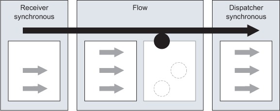
Table 11.3. Pros and cons of the fully synchronous mode

Pros	Cons
Supports transaction propagation	All load handled by the connector’s receiver threads
Simple to implement	Doesn’t use SEDA queueing

As noted earlier, using an outbound endpoint with a request-response exchange will cause the dispatcher to act synchronously. In that case, an asynchronously called flow can end up dispatching synchronously, using a thread from the flow thread pool for that end. This is illustrated in figure 11.8. This can also occur if the flow uses the event context (see section 12.1.1) to perform a synchronous dispatch programmatically. Look at table 11.4 for a summary of the pros and cons of this threading model.

Figure 11.8. If only the dispatcher is synchronous, the receiver thread is used up to the flow in which a thread is taken from the pool and used throughout the dispatcher.

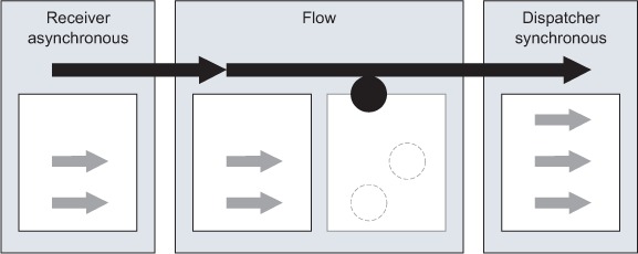
Table 11.4. Pros and cons of the asynchronous-synchronous mode

Pros	Cons
Allows synchronous routing in the dispatcher (as with a chaining router)	Can’t return the component response to the caller
Receiving decoupled from dispatching and servicing	Flow thread pool size constrains the outbound dispatching load capacity

Best practice

Use the request-response message exchange pattern on endpoints sparingly and only when it’s justified.

As you’ve learned, the default usage of the thread pools that can be involved in the processing of a message depends on the message exchange patterns being used and whether or not the flow is transactional. There will be times, however, when you’ll want to override this behavior, for instance, to force an otherwise asynchronous flow to be synchronous. You’ll see how to accomplish that in section 11.3. We’ll now look at how transports can also directly influence the thread pools’ usage.

11.2.2. Transport peculiarities

Transports can influence the threading model mostly in the way they handle incoming messages. In this section, we’ll detail some of these aspects for a few transports. This will give you a few hints about what to look for; we still recommend that you study the threading model of the transports you use in your projects if you decide you want to tune them.

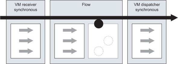
The first peculiarity we’ll look at is illustrated in figure 11.9. It’s possible for a message event to be fully processed in a flow without using any thread from any of its existing pools. Why? This can happen when you use the VM transport because, since it’s an in-memory protocol, Mule optimizes the event-processing flow for synchronous flow by piggybacking the same thread across flows. This allows, for example, a message to be transactionally processed across several flows by the same thread.

Figure 11.9. A fully synchronous flow using the VM transport can piggyback an incoming thread for event processing.

Some transports, such as HTTP or file, support the notion of polling receivers. Keep in mind that if you activate this feature, the poller will permanently borrow a thread from the receiver pool of the connector, as illustrated in figure 11.10. Because you can configure several connectors for the same transport, it’s a good idea to have a connector dedicated to polling and one or several other connectors for normal message processing.

Figure 11.10. A polling receiver permanently borrows a thread from the transport’s receiver pool.

Other transports don’t rely on a thread pool directly handled by Mule, as shown in figure 11.11. With the JMS transport, for instance, only the creation of receiver threads is handled by the JMS client infrastructure. In this case, Mule remains in control of these threads via its pool of JMS message listeners.^[2]

² The pool of JMS dispatcher threads is still fully controlled by Mule.

Figure 11.11. Some transports have their own receiver thread pool handled outside of Mule’s infrastructure.

In the introduction to this section, we mentioned the existence of a buffer for each thread pool. Similarly, certain transports natively support the notion of a request backlog that can accumulate requests when Mule isn’t able to handle them immediately, as shown in figure 11.12. For example, the TCP and HTTP transports can handle this situation gracefully by stacking incoming requests in their specific backlogs. Other transports, such as JMS or VM (with queuing activated), can also handle a pool-exhausted situation in a clean manner because they naturally support the notion of queues of messages.

Figure 11.12. Some transports support the notion of a request backlog used when the receiver thread pool is exhausted.

As you can see, transports can influence the way thread pools are used. The fact is that transports matter as far as threading is concerned. Therefore, it’s a good idea to spend some time understanding how the transports you use behave.

Best practice

Build a thorough understanding of the underlying protocols that you’re using through Mule’s transports.

Let’s now look at the different options Mule gives you for configuring these thread pools.

11.2.3. Tuning thread pools

Thread pools aren’t configured directly but via the configuration of threading profiles. Threading profiles are organized in a hierarchy of configuration elements whose scope varies from the most generic (Mule-level configuration) to the most specific (connector-level or flow-level). See figure 11.13.

Figure 11.13. Thread pools are configured via a hierarchy of profiles whose scope goes from the most generic to the most specific profile.

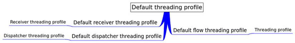
In this hierarchy, a profile defined at a lower (more specific) level overrides one defined at a higher (more generic) level. For example, consider the following configuration fragment:

<configuration>
  <default-threading-profile
    maxBufferSize="100" maxThreadsActive="20"
    maxThreadsIdle="10" threadTTL="60000"
    poolExhaustedAction="ABORT" />
</configuration>

This fragment defines a global threading profile that sets all the thread pools (receiver, dispatcher, and flow) to have by default a maximum number of active threads limited to 20 and a maximum number of idle threads limited to 10. It also defines that threads are deemed idle after a minute (60,000 milliseconds) of inactivity and that, in case of pool exhaustion (which means that the 100 spots in the buffer are used), any new request will be aborted and an exception will be thrown.

But what if a critical flow should never reject any request? You’d then override this Mule-wide default with a flow-level thread pool configuration, as shown in the following excerpt:

<flow name="CriticalService">
  ...
  <threading-profile
    maxBufferSize="100" maxThreadsActive="20"
    maxThreadsIdle="10" threadTTL="60000"
    poolExhaustedAction="RUN" />
</flow>

With this setting, the flow will never reject any incoming message, even if its thread pool is exhausted. It will, in fact, piggyback the incoming thread to perform the work, as it can’t hand it off to a thread from its own pool (this will tax the receiver’s thread pool, potentially creating problems there too). Note that you have to duplicate all the values defined in the global threading configuration, as there’s no way to inherit individual setting values.

Besides RUN and ABORT, the other supported exhausted actions are WAIT, which holds the incoming thread for a configurable amount of time until the pool accepts the event or a timeout occurs, and DISCARD and DISCARD_OLDEST, which silently drop the incoming event or the oldest one in the buffer, respectively.

You’re now probably wondering this: how do I size all these different thread pools? MuleSoft provides a comprehensive methodology for calculating these sizes^[3] based on four main factors: expected number of concurrent user requests, desired processing time, target response time, and acceptable timeout time. Before you follow that path, we’d like to draw your attention to the fact that for many deployments, the default values provided by Mule are all that’s needed. Unless you have specific requirements in one or several of these four factors, you’ll be better off most of the time leaving the default values in place. We encourage you to load test your configuration early on in your project and decide to tweak the thread pools only if you have evidence that you need to do so.^[4]

³ See http://mng.bz/zpr2 for more information.

⁴ By which we mean org.mule.transport.jms.MultiConsumerJmsMessageReceiver, not one of the polling message receivers that are also available.

Here are a few complementary tips:

• Use separate thread pools for administrative channels. For example, if you use TCP to remotely connect to Mule via a remote dispatcher agent (see section 12.2.2), use a specific connector for this TCP endpoint so it’ll have dedicated thread pools. That way, in case the TCP transport gets overwhelmed with messages, you’ll still be in a position to connect to Mule.
• Don’t forget the component pool. If you use component pooling, the object pool size must be commensurate to the flow thread pool size. It’s easy to define a global default thread pool size and forget to size a component pool accordingly.
• Pooled components decrease throughput. Pools of components are almost always less performant than singletons. Under load there will be contention of threads for objects in the pool. There’s also overhead in growing the pool. Use singleton components unless you have a good reason not to.
• Waiting is your worst enemy. The best way to kill the scalability of an application is to mobilize threads in long-waiting cycles. The same applies with Mule: don’t wait forever, and avoid waiting at all if it’s acceptable business-wise to reject requests that can’t be processed.

Mule offers total control over the thread pools it uses across the board for handling message events. You’re now better equipped to understand the role played by these pools, when they come into play, and what configuration factors you can use to tune them to your needs.

When a thread’s taken out of a pool, your main goal is to have this thread back in the pool as fast as possible. Let’s see how you can tune processing strategies to accomplish this.

11.2.4. Tuning processing strategies

Processing strategies, like thread pools, are also configurable. We discussed in section 11.2.1 how a processing strategy for a given flow is largely determined by the exchange patterns of the endpoints and whether or not a transaction’s in place. It’s possible, however, to explicitly set what the processing strategy for a given flow should be. This is done by setting the processingStrategy attribute on a flow, as illustrated next:

<flow processingStrategy="synchronous">
          <vm:inbound-endpoint path="in" exchange-pattern="one-way"/>
     <vm:outbound-endpoint path="out" exchange-pattern="one-way"/>
</flow>

By explicitly setting the processingStrategy for the above flow to synchronous, you tell Mule to bypass the default queued asynchronous behavior and use a single thread per every request.

Something we’ve glossed over until now is the flow thread pool. By now, hopefully it’s clear that a pool of threads exists in a receiver thread pool to consume messages and, optionally, a dispatcher thread pool to send messages. For message processors in between the message source and the outbound endpoint, Mule will borrow a thread from the flow thread pool to execute all message processors in that flow for a given message. This means all flow processing besides message reception and message dispatch occurs in a single thread.

Often, this behavior isn’t desirable. You saw an example at the beginning of this chapter of how the VM transport can be used to decompose message processing in a flow. That approach gives you the maximum amount of flexibility in that you have full control over tuning the receiving flow’s thread pools and processing strategies. Sometimes, however, you want to parallelize work across cores in your flow, but you don’t necessarily want to decouple everything with VM queues. In such situations, you can use the thread-per-processor-processing-strategy and the queued-thread-per-processor-processing-strategy.

The thread-per-processor-processing-strategy is the simpler of the two and ensures that, after the message source, each message processor in the flow processes the message in a separate thread. The queued-thread-per-processor-processing-strategy behaves identically, except that an internal SEDA queue is placed between each message processor, allowing you to introduce a buffer to hold messages when the flow thread pool is exhausted.

The following listing provides an alternative approach to tune listing 11.1 from the beginning of this chapter. Instead of using the VM transport, you use the queued-thread-per-processor-processing-strategy to ensure that the processing handled by each component of the flow occurs in its own thread.

Listing 11.3. Report processing in a single flow

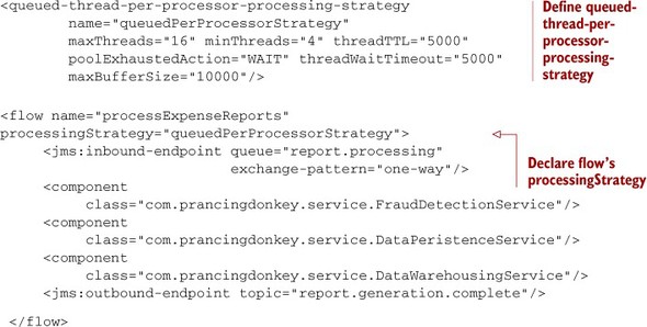
Listing 11.3 is a little bit different from the previous declaration of a flow’s processing strategy. In this case, you explicitly define the queued-thread-per-processor-processing-strategy, set some tuning parameters for it, and reference it from the flow. Similar namespace elements exist for the other processing strategies. At the time of writing, they include queued-thread-per-processor-processing-strategy, thread-per-processor-processing-strategy, asynchronous-processing-strategy, and queued-asynchronous-processing-strategy.

Declaring a global processing strategy using one of these elements provides two benefits. First, you can configure the processing strategy once and reference it from multiple flows. Second, you have the ability to tune the processing strategy using the attributes enumerated in table 11.5.

Table 11.5. Configuring a processing strategy

Name	Description
maxBufferSize	The maximum number of messages to queue when the thread pool is at capacity
maxThreads	The maximum number of threads that can be used
minThreads	The minimum number of threads to keep ready when the flow is idle
poolExhaustedAction	What to do when the thread pool runs out
threadTTL	How long to keep an inactive thread in the pool prior to evicting it
threadWaitTimeout	How long to wait for a thread when the poolExhaustedAction is WAIT

Custom processing strategies

You can write your own processing strategies by implementing org.mule.api.processor.ProcessingStrategy and defining a custom-processing-strategy element.

Processing strategies, combined with the receiver and dispatcher thread pool tuning you saw in the previous section, give you almost complete control over how Mule allocates threads for processing performance. This level of control often isn’t necessary; Mule’s out-of-the-box defaults for both receiver and dispatcher pools, as well as its processing strategy assumptions based on endpoints, are typically good enough for most scenarios. For high-throughput use cases, or use cases with special considerations such as slow consumers or performance-sensitive service components, some level of thread pool or processing strategy tuning is unavoidable.

In this section, you’ve seen approaches to tuning Mule and structuring Mule flows to achieve throughput. But knowing about these techniques isn’t worth anything unless you know where to apply them. Let’s take a look at how you can identify performance bottlenecks in Mule applications.

11.3. Identifying performance bottlenecks

Although threading profiles and processing strategies define the overall capacity of your Mule instance in terms of scaling and capacity, the performance of each moving part involved in processing each request will also impact the global throughput of your application. If the time needed to process each request is longer than the speed at which these requests come in, or if this time increases under load, you can end up in a position in which your thread pools will be exhausted no matter how many threads or how big a buffer you use.

Therefore, fine-grained performance matters. On the other hand, we all know Donald Knuth’s words of caution:^[5]

⁵ From “Structured Programming with go to Statements,” ACM Journal Computing Surveys. http://dl.acm.org/citation.cfm?id=356640.

We should forget about small efficiencies, say about 97% of the time: premature optimization is the root of all evil.

Should performance optimization be avoided entirely? No. Premature optimization is the issue. This encourages following a pragmatic approach to the question of increasing performances: build, measure, and correct.

Best practice

Don’t tune randomly; use a systematic approach to tuning.

Building has been the main focus of this book, so we consider that subject (hopefully) covered. In this section, we’ll first talk about gathering metrics to pinpoint performance pain. Then we’ll give some advice about what you can do based on these measures. This advice will be generic enough to guide you in the build phase—not in achieving premature optimization, but in making some choices that will reduce your exposure to performance issues.

Let’s start by looking at measuring performance issues with a profiler.

11.3.1. Profiler-based investigation

The most convenient way to locate places in an application that are good candidates for optimization (a.k.a. hot spots) is to use a profiler. As a Java-based application that can run on the most recent JVMs, and because its source code is available, Mule is transparent when it comes to profiling. To make things even easier, you can download a free Profiler Pack from www.mulesoft.org that contains the libraries required to profile a Mule instance with YourKit (http://yourkit.com). You still need to own a valid license from YourKit in order to analyze the results of a profiling session.

The way you activate the profiler depends on the way you deploy and start Mule (see section 8.1). With a standalone deployment, adding the -profile parameter to the startup command does the trick. If you deploy Mule in a Java EE container or bootstrap it from an IDE, you’ll have to refer to YourKit’s integration guidelines to have the profiler active.

To make the most of a profiling session, you’ll have to exercise Mule in a way that simulates its usage for the considered configuration. This will allow hot spots to be detected easily. You can use one of the test tools we’ll discuss in section 12.4 or create your own ad hoc activity generator if you have specific or trivial needs. Figure 11.14 shows YourKit’s memory dashboard while profiling the LoanBroker sample application that ships with Mule. This demonstration application comes with a client that can generate a hundred fake requests; we used it as a convenient ad hoc load injector able to exercise Mule in a way that’s realistic for the configuration under test.

Figure 11.14. Profiling Mule’s memory with YourKit while messages are being processed

What can you expect from such a profiling session? Covering the subject of Java application profiling is beyond the scope of this book, but here are a few key findings you can expect:

• Hot spots— Methods that are excessively called or unexpectedly slow
• Noncollectable objects— Lead to memory leaks
• Monitor locks— Excess can create contentions between threads
• Deadlocks— Can take down a complete application
• Excessive objects or threads creation— Can lead to unexpected memory exhaustion

Once you’ve identified areas of improvement, it’ll become possible to take corrective action. As far as profiling is concerned, a good strategy is to perform differential and incremental profiling sessions. This consists of first capturing a snapshot of a profiling session before you make any change to your configuration or code. This snapshot will act as a reference to which you will compare snapshots taken after each change. Whenever the behavior of your application has improved, you’ll use the snapshot of the successful session as the new reference. It’s better to make one change at a time and reprofile after each change; otherwise, you’ll have a hard time telling what the cause was for an improvement or a degradation.

The LoanBroker sample application that we’ve already profiled comes with several configuration flavors. We’ve compared the profiles of routing-related method invocations of this application running in asynchronous and synchronous modes. The differences, which are shown in figure 11.15, confirm the impact of the configuration change: the asynchronous version depends more on inbound routing and filtering, whereas the synchronous one uses the response routers for quotes aggregation.

Figure 11.15. Comparing two profiling session snapshots helps determine the impact of configuration changes.

YourKit Compatibility

The Profiler Pack and the Profiler Agent are packaged for a particular version of YourKit. Be sure to check that they’re compatible with the version you own. If you use a different version and don’t want to upgrade or downgrade to the version supported by Mule’s extensions, you’ll have to use the libraries that are shipped with your version of YourKit in lieu of the ones distributed by MuleSoft.

Using a profiler is the best way to identify performance-challenged pieces of code. But whether you use a profiler or not, there are general guidelines that you can apply to your Mule projects. We’ll go through them now.

11.3.2. Performance guidelines

Whether you’ve used a profiler or not, this section offers a few pieces of advice about coding and configuring your Mule applications for better performance. You’ll see that some of this advice is generic, whereas some is Mule-specific.

Follow good middleware coding practices

Mule-based applications don’t escape the rules that apply to middleware development. This may sound obvious, but it’s not. It’s all too easy to consider a Mule project as being different from, say, a standard Java EE one because far less code is involved (or it’s all in scripts). The reality is that the same best practices apply. Let’s name a few:

• Use appropriate algorithms and data structures.
• Write sound concurrent code in your components or transformers (thread-safety, concurrent collections, no excessive synchronization, and so on).
• Consider caching.
• Avoid generating useless garbage (favor singleton-scoped beans over prototypes).

Reduce busywork

Be aware that inefficient logging configuration can severely harm performance. Reduce verbosity in production and activate only the relevant appenders (for example, if you only need FILE, there’s no need to configure CONSOLE). In the same vein, don’t go overboard with your usage of notifications. If you activate all the possible families of notifications (see section 12.3.3), a single message can fire multiple notifications while it’s being processed in Mule, potentially flooding your message listening infrastructure. You certainly don’t need to expose your application to a potential internal self-denial of service.

Use efficient message routing

Message routing is an important part of what keeps a Mule instance busy; therefore, it doesn’t hurt to consider performance when configuring your routers and filters. For example, avoid delivering messages to a component if you know it will ignore it. Doing so will also save you the time spent in the component interceptor stack and the entry point resolvers.

Best practice

Investigate high-performance message processors such as SXC or Smooks if you intend to perform processing or transformation on messages with huge payloads.

Carry lighter payloads

Carrying byte-heavy payloads creates a burden both in memory usage and in processing time. Mule offers different strategies to alleviate this problem, and these strategies mostly depend on the transport you use. Here’s an incomplete list of possible options to consider:

• The file transport can receive java.io.File objects as the message payload instead of the whole file content, allowing you to carry a light object until the real processing needs to happen and the file content needs to be read.
• Some transports can receive incoming request content as streams instead of arrays of bytes, either by explicitly configuring them for streaming or by virtue of the incoming request. This is a powerful option for dealing with huge payloads, but you’ll have to be careful with the synchronicity of the different parts involved in the request processing (see section 11.2.1), as you can end up with a closed input stream being dispatched if the receiver wasn’t synchronously bound to the termination of the processing phase.
• You can opt to return streams from your components that produce heavy payloads. Many transports can accept streams and serialize them to bytes at the latest possible stage of the message-dispatching process. In the worst case, you can always use an existing transformer to deal with the stream serialization (see section 4.3.1).
• The Claim Check pattern (documented here: http://eaipatterns.com/Store-InLibrary.html) can be used to store a reference to the message payload in an external source. This allows it to be loaded on demand rather than being passed around in the message. An example of this would be to use a database row ID as the payload of the message and use this to selectively load the data, or parts of the data, into Mule when it’s necessary for processing.

Tune transports

As we discussed in section 11.2.2, transports have their own characteristics that can influence threading and, consequently, performance. The general advice about this is that you should know the transports you use and how they behave. You should look for timeout parameters, buffer sizes, and delivery optimization parameters (such as keep alive and send no delay for TCP and HTTP, chunking for HTTP, or DUPS_OK _ACKNOWLEDGE for nontransactional JMS).

Best practice

For HTTP inbound endpoints, you should prefer the Jetty transport in standalone deployments and the servlet transport in embedded deployment over the default HTTP transport.

Tune Mule’s JVM

Finally, because Mule is a Java application, tuning the JVM on which it runs can also contribute to increasing performance. Mule’s memory footprint is influenced by parameters such as the number of threads running or the size of the payloads you carry as bytes (as opposed to streams). Right-sizing Mule’s JVM and tuning its garbage collector or some other advanced parameters can effectively be achieved by running load tests and long-running tests that simulate the expected traffic (sustained and peak).

Performance tuning is the kingdom of YMMV;^[6] there’s no one-size-fits-all solution for such a domain. In this section, we’ve given you some hints on how to track down performance bottlenecks with a profiler and some advice you can follow to remedy these issues.

⁶ Your Mileage May Vary.

11.4. Summary

In this chapter, we investigated the notions of thread pools and performance optimization. We talked about how synchronicity deeply affects the way threading occurs in Mule. We left you with a lot of different options to tune the different thread pools to your needs. We also presented a pragmatic approach to performance optimization with the help of a profiler and gave you a handful of general tips for better use of your system’s available resources (memory and CPU).

Part 1 of this book covered the basics of Mule: working with flows, using connectors and components, and routing and transforming data. That laid the groundwork for part 2, designed to give you confidence in deploying, securing, and tuning Mule applications, and handling errors. In part 3 we’ll turn our attention to Mule’s API, which lets you go “under the hood” of Mule applications and fully harness its flexibility.