The first step is to define the configuration parameter for the MLP classifier, is as follows:

val path = "resources/data/chap9/"
val ALPHA = 0.5; val ETA = 0.03
val NUM_EPOCHS = 250; val EPS = 1.0e-6
var hidLayers = Array[Int](7, 7)  //1

var config = MLPConfig(ALPHA, ETA, hidLayers, NUM_EPOCHS, EPS)

Besides the learning parameters, the network is initialized with two configurations:

Next, let's create the search space of the prices of all the ETFs used in the analysis:

val symbols = Array[String]("FXE", "FXA", "SPY", "GLD", "FXB", "FXF", "FXC", "FXY", "CYB") //2

The closing prices of all the ETFs over a period of three years are extracted from the Google Financial tables, using the GoogleFinancials extractor (line 3) for a basket of ETFs (line 2):

val prices = symbols.map(s =>DataSource(s"$path$s.csv",true))
                    .map( _ |> GoogleFinancials.close) //3
                    .map( _.toArray)

The next step consists of implementing the mechanism to extract the target and the features from a basket of ETFs, or studies introduced in the previous paragraph. Let's consider the following study as the list of ETF ticker symbols (line 4):

val study = Array[String]("FXE", "FXF", "FXB", "CYB") //4

The first element of the study, FXE, is the labeled output; the remaining three elements are observed features. For this study, the network architecture has three input variables {FXF, FXB, CYB} and one output variable FXE:

val obs = study.map(s =>index.get(s).get).map( prices( _ )) //5
val features = obs.drop(1).transpose //6
val target = Array[DblVector](obs(0)).transpose  //7

The set of observations is built using an index (line 5). By convention, the first observation is selected as the label data and the remaining studies as the features for training. As the observations are loaded as an array of time series, the time features of series is computed through transpose (line 6). The single output variable, target, has to be converted into a matrix before transposition (line 7).

Ultimately, the model is built through instantiation of the MLP class:

val THRESHOLD = 0.08
implicit val mlpObjective = new MLP. MLPBinClassifier
val mlp = MLP[Double](config, features, target)
mlp.accuracy(THRESHOLD)

The objective type, mlpObjective, is implicitly defined as an MLP binary classifier, MLPBinClassifier. The square root of the sum of squares of the difference between the predicted output generated by the MLP and the target value is computed and compared to a predefined threshold. The accuracy value is computed as the percentage of data points, whose prediction matches the target value within a range < THRESHOLD:

val nCorrects = xt.toArray.zip(labels).foldLeft(0)((s, xtl) => {
   val output = model.get.getOutput(xtl._1) //8
   val _sse = xtl._2.zip(output.drop(1))
                    .foldLeft(0.0)((err,tp) => { 
                       val diff= tp._1 - tp._2
                       err + diff*diff
                    }) //9
   val error = Math.sqrt(_sse)/(output.size-1) //10
   if(error < threshold) s + 1
   else s
})
nCorrects.toDouble/xt.size

The implementation of the computation of the accuracy, as in the previous code snippet, retrieves the values of the output layer (line 8). The error value (line 10) is computed as the square root of the sum of squared errors, _sse (line 9). Finally, a prediction is considered correct if it is equal to the labeled output, within the margin error, threshold.

The test consists of evaluating six different models to determine which ones provide the most reliable correlation. It is critical to ensure that the result is somewhat independent of the architecture of the neural network. Different architectures are evaluated as part of the test.

The following charts compare the models for two architectures:

This first chart visualizes the accuracy of the six regression models with an architecture consisting of a variable number of inputs [2, 7], one output variable, and two hidden layers of four nodes each. The features (ETF symbols) are listed on the left-hand side of the arrow => along the y-axis. The symbol on the right-hand side of the arrow is the expected output value:

Accuracy of MLP with two hidden layers of four nodes each

The next chart displays the accuracy of the six regression models for an architecture with three hidden layers of eight, five, and six nodes, respectively:

Accuracy of MLP with three hidden layers with 8, 5, and 6 nodes, respectively

The two network architectures shared a lot of similarity: in both cases, the most accurate regression models are as follows:

On the other hand, the prediction the Canadian dollar to US dollar's exchange rate (FXC) using the exchange rate for the Japanese yen (FXY) and the Australian dollar (FXA) is poor with both configuration.

The next test consists of evaluating the impact of the hidden layer(s) of configuration on the accuracy of three models: (FXF, FXB, CYB => FXE), (FCX, GLD, FXA =>FXY), and (FXC, GLD, FXA, FXY, FXB => FXE). For this test, the accuracy is computed by selecting a subset of the training data as a test sample, for the sake of convenience. The objective of the test is to compare different network architectures using some metrics, not to estimate the absolute accuracy of each model.

The four network configurations are as follows:

The complex neural network architecture with two or more hidden layers generates weights with similar accuracy. The four-node single hidden layer architecture generates the highest accuracy. The computation of the accuracy using a formal cross-validation technique would generate a lower accuracy number.

Finally, we look at the impact of the complexity of the network on the duration of the training, as in the following graph:

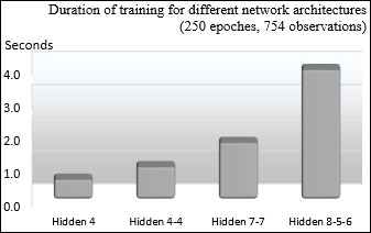
Impact of hidden layers architecture on duration of training

Not surprisingly, the time complexity increases significantly with the number of hidden layers and number of nodes.