
This chapter presents the concept of reinforcement learning, which is widely used in gaming and robotics. The second part of this chapter is dedicated to learning classifier systems, which combine reinforcement learning techniques with evolutionary computing introduced in the previous chapter. Learning classifiers are an interesting breed of algorithms that are not commonly included in literature dedicated to machine learning. I highly recommend you to read the seminal book on reinforcement learning by R. Sutton and A. Barto [11:1] if you are interested to know about the origin, purpose, and scientific foundation of reinforcement learning.
In this chapter, you will learn the following:
The section on learning classifier systems (LCS) is mainly informative and does not include a test case.
The need of an alternative to traditional learning techniques arose with the design of the first autonomous systems.
Autonomous systems are semi-independent systems that perform tasks with a high degree of autonomy. Autonomous systems touch every facet of our life, from robots and self-driving cars to drones. Autonomous devices react to the environment in which they operate. The reaction or action requires the knowledge of not only the current state of the environment but also the previous state(s).
Autonomous systems have specific characteristics that challenge traditional methodologies of machine learning, as listed here:
- Autonomous systems have poorly defined domain knowledge because of the sheer number of possible combinations of states.
- Traditional non-sequential supervised learning is not a practical option because of the following:
- Training consumes significant computational resources, which are not always available on small autonomous devices
- Some learning algorithms are not suitable for real-time prediction
- The models do not capture the sequential nature of the data feed
- Sequential data models such as hidden Markov models require training sets to compute the emission and state transition matrices (as explained in the The hidden Markov model (HMM) section in Chapter 7, Sequential Data Models), which are not always available. However, a reinforcement learning algorithm benefits from a hidden Markov model in case some of the states are unknown. These algorithms are known as behavioral hidden Markov models [11:2].
- Genetic algorithms are an option if the search space can be constrained heuristically. However, genetic algorithms have unpredictable response time, which makes them impractical for real-time processing.
Reinforcement learning is an algorithmic approach to understanding and ultimately automating goal-based decision-making. Reinforcement learning is also known as control learning. It differs from both supervised and unsupervised learning techniques from the knowledge acquisition standpoint: autonomous, automated systems or devices learn from direct, real-time interaction with their environment. There are numerous practical applications of reinforcement learning from robotics, navigation agents, drones, adaptive process control, game playing, and online learning, to schedule and routing problems.
Reinforcement learning introduces a new terminology as listed here, quite different from that of older machine learning techniques:
- Environment: The environment is any system that has states and mechanisms to transition between states. For example, the environment for a robot is the landscape or facility it operates in.
- Agent: The agent is an automated system that interacts with the environment.
- State: The state of the environment or system is the set of variables or features that fully describe the environment.
- Goal or absorbing state or terminal state: A goal state is the state that provides a higher discounted cumulative rewards than any other state. It is a constraint on the training process that prevents the best policy from being dependent on the initial state.
- Action: An action defines the transition between states. The agent is responsible for performing or at least recommending an action. Upon execution of the action, the agent collects a reward or punishment from the environment.
- Policy: The policy defines the action to be selected and executed for any state of the environment.
- Best policy. This is the policy generated through training. It defines the model in Q-learning and is constantly updated with any new episode.
- Reward: A reward quantifies the positive or negative interaction of the agent with the environment. Rewards are essentially the training set for the learning engine.
- Episode: This defines the number of steps necessary to reach the goal state from an initial state. Episodes are also known as trials.
- Horizon: The horizon is the number of future steps or actions used in the maximization of the reward. The horizon can be infinite, in which case the future rewards are discounted in order for the value of the policy to converge.
The key component in reinforcement learning is a decision-making agent that reacts to its environment by selecting and executing the best course of actions and being rewarded or penalized for it [11:3]. You can visualize these agents as robots navigating through an unfamiliar terrain or a maze. Robots use reinforcement learning as part of their reasoning process after all. The following diagram gives the overview architecture of the reinforcement learning agent:

The agent collects the state of the environment, selects, and then executes the most appropriate action. The environment responds to the action by changing its state and rewarding or punishing the agent for the action.
The four steps of an episode or learning cycle are as follows:
- The learning agent either retrieves or is notified of a new state of the environment.
- The agent evaluates and selects the action that may provide the highest reward.
- The agent executes the action.
- The agent collects the reward or penalty and applies it to calibrate the learning algorithm.
The action of the agent modifies the state of the system, which in turn notifies the agent of the new operational condition. Although not every action will trigger a change in the state of the environment, the agent collects the reward or penalty nevertheless. At its core, the agent has to design and execute a sequence of actions to reach its goal. This sequence of actions is modeled using the ubiquitous Markov decision process (refer to the Markov decision processes section in Chapter 7, Sequential Data Models.)
Tip
Dummy actions
It is important to design the agent so that actions may not automatically trigger a new state of the environment. It is easy to think about a scenario in which the agent triggers an action just to evaluate its reward without affecting the environment significantly. A good metaphor for such a scenario is the rollback of the action. However, not all environments support such a dummy action, and the agent may have to run Monte-Carlo simulations to try out an action.
Reinforcement learning is particularly suited to problems for which long-term rewards can be balanced against short-term rewards. A policy enforces the trade-off between short-term and long-term rewards. It guides the behavior of the agent by mapping the state of the environment to its actions. Each policy is evaluated through a variable known as the value of policy.
Intuitively, the value of a policy is the sum of all the rewards collected as a result of the sequence of actions taken by the agent. In practice, an action over the policy farther in the future obviously has a lesser impact than the next action from state St to state St+1. In other words, the impact of future actions on the current state has to be discounted by a factor, known as the discount coefficient for future rewards < 1.
Tip
State transition matrix
The state transition matrix has have been introduced in the The hidden Markov model section in Chapter 7, Sequential Data Models.
The optimum policy, ![]() *, is the agent's sequence of actions that maximizes the future reward discounted to the current time.
*, is the agent's sequence of actions that maximizes the future reward discounted to the current time.
The following table introduces the mathematical notation of each component of reinforcement learning:
|
Notation |
Description |
|---|---|
|
S = {si} | |
|
A = {ai} |
Actions on the environment |
|
Πt = p(at|st) |
Policy (or strategy) of the agent |
|
Vπ(st) |
Value of the policy at the state |
|
pt =p(st+1|st,at) |
State transition probabilities from state st to state st+1 |
|
rt= p(rt+1|st,st+1,at) |
Reward of an action at for a state st |
|
Rt |
Expected discounted long term return |
|
γ |
Coefficient to discount the future rewards |
The purpose is to compute the maximum expected reward, Rt, from any starting state, sk, as the sum of all discounted rewards to reach the current state, st. The value ![]() of a policy
of a policy ![]() at state st is the maximum expected reward Rt given the state st.
at state st is the maximum expected reward Rt given the state st.

The problem of finding the optimal policies is indeed a nonlinear optimization problem whose solution is iterative (dynamic programming). The expression of the value function ![]() of a policy
of a policy ![]() can be formulated using the Markovian state transition probabilities pt.
can be formulated using the Markovian state transition probabilities pt.
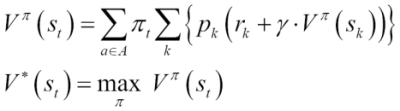
V*(st) is the optimal value of state st across all the policies. The equations are known as the Bellman optimality equations.
Note
The curse of dimensionality
The number of states for a high-dimension problem (large-feature vector) becomes quickly insolvable. A workaround is to approximate the value function and reduce the number of states by sampling. The application test case introduces a very simple approximation function.
If the environment model, state, action, and rewards, as well as transition between states, are completely defined, the reinforcement learning technique is known as model-based learning. In this case, there is no need to explore a new sequence of actions or state transitions. Model-based learning is similar to playing a board game in which all combinations of steps necessary to win are completely known.
However, most practical applications using sequential data do not have a complete, definitive model. Learning techniques that do not depend on a fully defined and available model are known as model-free techniques. These techniques require exploration to find the best policy for any given state. The remaining sections in this chapter deal with model-free learning techniques, and more specifically the temporal difference algorithm.
Temporal difference is a model-free learning technique that samples the environment. It is a commonly used approach to solve the Bellman equations iteratively. The absence of a model requires a discovery or exploration of the environment. The simplest form of exploration is to use the value of the next state and the reward defined from the action to update the value of the current state, as described in the following diagram:

Illustration of the temporal difference algorithm
The iterative feedback loop used to adjust the value action on the state plays a role similar to back propagation of errors in artificial neural networks or minimization of the loss function in supervised learning. The adjustment algorithm has to:
-
Discount the estimate value of the next state using the discount rate

-
Strike a balance between the impacts of the current state and the next state on updating the value at time t using the learning rate

The iterative formulation of the first Bellman equation predicts ![]() (st), the value function of state st from the value function of the next state st+1. The difference between the predicted value and the actual value is known as the temporal difference error abbreviated as
(st), the value function of state st from the value function of the next state st+1. The difference between the predicted value and the actual value is known as the temporal difference error abbreviated as ![]() t.
t.

An alternative to evaluating a policy using the value of the state, ![]() (st), is to use the value of taking an action on a state st known as the value of action (or action-value)
(st), is to use the value of taking an action on a state st known as the value of action (or action-value) ![]() (st, at).
(st, at).
There are two methods to implement the temporal difference algorithm:
Let's consider the temporal difference algorithm using an off-policy method and its most commonly used implementation: Q-learning.
Q-learning is a model-free learning technique using an off-policy method. It optimizes the action-selection policy by learning an action-value function. Like any machine learning technique that relies on convex optimization, the Q-learning algorithm iterates through actions and states using the quality function, as described in the following mathematical formulation.
The algorithm predicts and discounts the optimum value of action, max{Qt}, for the current state st and action at on the environment to transition to state st+1.
Similar to genetic algorithms that reuse the population of chromosomes in the previous reproduction cycle to produce offspring, the Q-learning technique strikes a balance between the new value of the quality function Qt+1 and the old value Qt using the learning rate, ![]() . Q-learning applies temporal difference techniques to the Bellman equation for an off-policy methodology.
. Q-learning applies temporal difference techniques to the Bellman equation for an off-policy methodology.

A value 1 for the learning rate ![]() discards the previous state, while a value 0 discards learning. A value 1 for the discount rate
discards the previous state, while a value 0 discards learning. A value 1 for the discount rate ![]() uses long-term rewards only, while a value 0 uses the short-term reward only.
uses long-term rewards only, while a value 0 uses the short-term reward only.
Q-learning estimates the cumulative reward discounted for future actions.
Let's apply our hard-earned knowledge of reinforcement learning to management and optimization of a portfolio of exchange-traded funds.
Let us implement the Q-learning algorithm in Scala.
The key components of the implementation of the Q-learning algorithm are as follows:
- The
QLearningclass implements training and prediction methods. It defines a data transformation by implementing thePipeOperatortrait. The constructor has three arguments: a configuration of typeQLConfig, a search space of typeQLSpace, and a mutable policy of typeQLPolicy. - The
QLSpaceclass has two components: a sequence of states of typeQLStateand the ID of one or more goal states within the sequence. - A state,
QLState, contains a sequence ofQLActioninstances used in its transition to another state. - The model of type
QLModelis generated through training. It contains the best policy and the accuracy for a model.
The following diagram shows the flow of the Q-learning algorithm:

The QLAction class specifies the transition of one state with ID from to another state with ID to, as shown here:
class QLAction[T <% Double](val from: Int, val to: Int)
Actions have a Q value (or action-value), a reward, and a probability. The implementation defines these three values in three separate matrices: Q for the action values, R for rewards, and P for probabilities, in order to stay consistent with the mathematical formulation.
A state of type QLState is fully defined by its ID, the list of actions to transition to some other states, and a property prop of parameterized type, as shown in the following code:
class QLState[T](val id: Int, val actions: List[QLAction[T]=List.empty, val prop: T])
The state might not have any actions. This is usually the case of the goal or absorbing state. In this case, the list is empty. The parameterized prop property is a placeholder for any information, heuristic about the state, or any action performed by the state.
The next step consists of creating the graph or search space.
The search space is the container responsible for any sequence of states. The QLSpace class takes the following parameters:
- The sequence of all the possible
states - The ID of one or several states that have been selected as
goals
The QLSpace class can be implemented as follows:
class QLSpace[T](states: Seq[QLState[T]], goals: Array[Int]) {
   val statesMap = states.map(st => (st.id, st)).toMap //1
   val goalStates = new HashSet[Int]() ++ goals //2

   def maxQ(state: QLState[T], policy: QLPolicy[T]): Double //3
   def init(r: Random) = states(r.nextInt(states.size-1)) //4
   def nextStates(st: QLState[T]): List[QLState[T]] //5
   …
}
The instantiation of the QLSpace class generates a map, statesMap, to retrieve the state using its id (line 1) and the set of goals, goalStates (line 2). Furthermore, the maxQ method computes the maximum action-value, maxQ, for a state given a policy (line 3), the init method selects an initial state for training episodes (line 4), and finally, the nextStates method retrieves the list of states resulting from the execution of all the actions associated to the st state (line 5).
The search space is actually created by the instance factory defined in the QLSpace companion object, as shown here:
def apply[T](numStates: Int, goals: Array[Int], features: Set[T], neighbors: (Int, Int) => List[Int]): QLSpace[T] = {
  val states = features
               .zipWithIndex
               .map(x => {
                  val actions = neighbors(x._2, numStates)
                                .map(j => QLAction[T](x._2,j))
                                .filter(x._2 != _.to)
                   QLState[T](x._2, actions, x._1
               })
  new QLSpace[T](states.toArray, goals)
}
The apply method creates a list of states using the features set as input. Each state creates its list of actions. The user-defined function, neighbors, constrains the number of actions assigned to each state. The test case describes a very simple implementation of the neighbors function, which is defined in the configuration.
Each action has an action-value, a reward, and a potentially probability. The probability variable is introduced to model simply the hindrance or adverse condition for an action to be executed. If the action does not have any external constraint, the probability is 1. If the action is not allowed, the probability is 0.
Tip
Dissociating policy from states
The action and states are the edges and vertices of the search space or search graph. The policy defined by the action-value, rewards, and probabilities is completely dissociated from the graph. The Q-learning algorithm initializes the reward matrix and updates the action-value matrix independently of the structure of the graph.
The QLData class is a container for three variables: reward, probability, and value for the Q-value, as shown here:
class QLData(var reward: Double = 1.0, var probability: Double = 1.0 var value: Double = 0.0) {
   def estimate: Double = value*probability
}
The estimate method adjusts the Q-value, value, with the probability to reflect any external condition that can impede the action.
Tip
Mutable data
You might wonder why the QLData class uses variables instead of values as recommended by the best Scala coding practices [11:4]. An instance of an immutable class would be created for each action or state transition. The training of the Q-learning model entails iterating across several episodes, each episode being defined as a multiple iteration. For instance, the training of a model with 400 states for 10 episodes of 100 iterations can potentially create 160 million instances of QLData. Although not quite elegant, mutability reduces the load on the JVM garbage collector.
Next, let us create a simple schema or class, QLInput, to initialize the reward and probability associated with each action as follows:
class QLInput(val from: Int, val to: Int, val reward: Double =1.0, val probability: Double =1.0)
The first two arguments are the identifiers for the source state, from, and target state, to, for this specific action. The last two arguments are the reward, collected at the completion of the action, and its probability. There is no need to provide an entire matrix. Actions have a reward of 1 and a probability of 1 by default. You only need to create an input for actions that have either a higher reward or a lower probability.
The number of states and a sequence of input define the policy of type QLPolicy. It is merely a data container, as shown here:
class QLPolicy[T](numStates: Int, input: Array[QLInput]) {
  val qlData = {
     val data = Array.tabulate(numStates)(v =>
                           Array.fill(numStates)(new QLData[T]))
     input.foreach(i => {
        data(i.from)(i.to).reward = i.reward //1
        data(i.from)(i.to).probability = i.probability //2
     })
     data
  }
  …
The constructor initializes the qlData matrix of type QLData with the input data, reward (line 1) and probability (line 2). The QLPolicy class defines the methods of the element in the reward (line 3), probability, and Q-learning action-value (line 4) matrices as follows:
def R(from: Int, to: Int): Double = qlData(from)(to).reward  //3
def Q(from: Int, to: Int): Double = qlData(from)(to).value  //4
The QLearning class encapsulates the Q-learning algorithm, and more specifically the action-value updating equation. It implements PipeOperator to the prediction used as a transformation between states, as shown here:
class QLearning[T](config: QLConfig, qlSpace: QLSpace[T],qlPolicy: QLPolicy[T]) extends PipeOperator[QLState[T], QLState[T]]
The constructor takes the following parameters:
- Configuration of the algorithm,
config - Search space,
qlSpace - Policy,
qlPolicy
The model is generated or trained during the instantiation of the class (refer to the Design template for classifier section in Appendix A, Basic Concepts.)
The configuration defines the learning rate, alpha; the discount rate, gamma the maximum number of states (or length) of an episode, episodeLength; the number of episodes used in training, numEpisodes; the minimum coverage of the state transition/actions during training to select the best policy, minCoverage; and the search constraint function, neighbors, as shown here:
class QLConfig(val alpha: Double, val gamma: Double, val episodeLength: Int, val numEpisodes: Int, val minCoverage: Double, val neighbors: (Int, Int) => List[Int]) extends Config
Let us look at the computation of the best policy during training. First, we need to define a model class, QLModel, with the best policy and its state-transition coverage of training as parameters:
class QLModel[T](val bestPolicy: QLPolicy[T], val coverage:Double)
The creation of model consists of executing multiple episodes to extract the best policy. Each episode starts with a randomly selected state, as shown in the following code:
val model: Option[QLModel[T]] = {
  val r = new Random(System.currentTimeMillis) //1
  val rg = Range(0, config.numEpisodes)
  val cnt =rg.foldLeft(0)((s, _) => s+(if(train(r)) 1 else 0))//2

  val accuracy = cnt.toDouble/config.numEpisodes
  if( accuracy > config.minCoverage )
     Some(new QLModel[T](qlPolicy, coverage)) //3
  else None
}
The model initialization code creates a random number generator (line 1), and iterates the generation of the best policy starting from a randomly selected state config.numEpisodes times (line 2). The transition coverage is computed as the percentage of times the search ends with the goal state (line 3). The initialization succeeds only if the accuracy exceeds a threshold value, config.minCoverage, specified in the configuration.
Tip
Quality of the model
The implementation uses the coverage to measure the quality of the model or best policy. The F1 measure (refer to the Assessing a model section in Chapter 2, Hello World!), is not appropriate because there are no false positives.
The train method does the heavy lifting at each episode. It triggers the search by selecting the initial state using a random generator r with a new seed, as shown in the following code:
def train(r: Random): Boolean =  {
   r.setSeed(System.currentTimeMillis*Random.nextInt)
   qlSpace.isGoal(search((qlSpace.init(r), 0))._1)
}
The implementation of search for the goal state(s) from any random states is a textbook implementation of the Scala tail recursion.
Tail recursion is a very effective construct to apply an operation to every item of a collection [11:5]. It optimizes the management of the function stack frame during the recursion. The annotation triggers a validation of the condition necessary for the compiler to optimize the function calls, as shown here:
@scala.annotation.tailrec
def search(st: (QLState[T], Int)): (QLState[T], Int) = {
  val states = qlSpace.nextStates(st._1) //1

  if( states.isEmpty || st._2 >= config.episodeLength ) st //2
  else {
    val state = states.maxBy(s => qlPolicy.R(st._1.id,s.id ))//3

    if( qlSpace.isGoal(state) ) (state, st._2) //4
    else {
      val r = qlPolicy.R(st._1.id, state.id)
      val q = qlPolicy.Q(st._1.id, state)  //5
      val nq = q + config.alpha*(r + config.gamma *
                           qlSpace.maxQ(state, qlPolicy) - q)//6
      qlPolicy.setQ(st._1.id, state.id, nq) //7
      search((state, st._2))
    }
  }
}
Let us dive into the implementation for the Q action-value updating equation. The recursion uses the tuple (state, iteration number in the episode) as argument. First, the recursion invokes the nextStates method of QLSpace to retrieve all the states associated with the current state, st, through its actions, as shown here:
def nextStates(st: QLState[T]): List[QLState[T]] =
    st.actions.map(ac => statesMap.get(ac.to).get )
The search completes and returns the current state if either the length of the episode (maximum number of states visited) is reached or the goal is reached or there is no further state to transition to (line 2). Otherwise the recursion computes the state to which the transition generates the higher reward R from the current policy (line 3). The recursion returns the state with the highest reward if it is one of the goal states (line 4). The method retrieves the current q action value and r reward matrices from the policy, and then applies the equation to update the action-value (line 6). The method updates the action-value Q with the new value nq (line 7).
The action-value updating equation requires the computation of the maximum action-value associated with the current state, which is performed by the maxQ method of the QLSpace class:
def maxQ(state: QLState[T], policy: QLPolicy[T]): Double = {
   val best = states.filter( _ != state)
                    .maxBy(st => policy.EQ(state.id, st.id))
   policy.EQ(state.id, best.id)
}
Note
Reachable goal
The algorithm does not require the goal state to be reached for every episode. After all, there is no guarantee that the goal will be reached from any randomly selected state. It is a constraint on the algorithm to follow a positive gradient of the rewards when transitioning between states within an episode. The goal of the training is to compute the best possible policy or sequence of states from any given initial state. You are responsible for validating the model or best policy extracted from the training set, independent from the fact that the goal state is reached for every episode.
The last functionality of the QLearning class is the prediction using the model created during training. The method predicts a state from an existing state.
def |> : PartialFunction[QLState[T], QLState[T]] = {
  case state: QLState[T] if(state != null && model != None)
      => nextState(state, 0)._1
}
The data transformation |> computes the best outcome, nextState, given a state using another tail recursion, as follows:
@scala.annotation.tailrec
def nextState(st: (QLState[T], Int)): (QLState[T], Int) =  {
   val states = qlSpace.nextStates(st._1)

   if( states.isEmpty || st._2 >= config.episodeLength)  st
   else nextState( (states.maxBy(s =>
               model.get.bestPolicy.R(st._1.id, s.id)), st._2+1))
}
The prediction ends when no more states are available or the maximum number of iterations within the episode is exceeded. You can define a more sophisticated exit condition. The challenge is that there is no explicit error or loss variable/function that can be used except the temporal difference error. The prediction returns either the best possible state, or None if the model cannot be created during training.
The Q-learning algorithm is used in many financial and market trading applications [11:6]. Let us consider the problem of computing the best strategy to trade certain types of options given some market conditions and trading data.
The Chicago Board Options Exchange (CBOE) offers an excellent online tutorial on options [11:7]. An option is a contract giving the buyer the right but not the obligation to buy or sell an underlying asset at a specific price on or before a certain date (refer to the Options trading section under Finances 101 in Appendix A, Basic Concepts.) There are several option pricing models, the Black-Scholes stochastic partial differential equations being the most recognized [11:8].
The purpose of the exercise is to predict the price of an option on a security for N days in the future according to the current set of observed features derived from the time to expiration, price of the security, and volatility. Let's focus on the call options of a given security, IBM. The following chart plots the daily price of IBM stock and its derivative call option for May 2014 with a strike price of $190:

The price of an option depends on the following parameters:
- Time to expiration of the option (time decay)
- The price of the underlying security
- The volatility of returns of the underlying asset
Pricing model usually does not take into account the variation in trading volume of the underlying security. So it would be quite interesting to include it in our model. Let us define the state of an option using the following four normalized features:
- Time decay: This is the time to expiration once normalized over [0, 1].
- Relative volatility: This is the relative variation of the price of the underlying security within a trading session. It is different from the more complex volatility of returns defined in the Black-Scholes model, for example.
- Volatility relative to volume: This is the relative volatility of the price of the security adjusted for its trading volume.
- Relative difference between the current price and strike price: This measures the ratio of the difference between price and strike price to the strike price.
The following graph shows the four normalized features for IBM option strategy:

The implementation of the option trading strategy using Q-learning consists of the following steps:
Let us select N =2 as the number of days in the future for our prediction. Any longer-term prediction is quite unreliable because it falls outside the constraint of the discrete Markov model. Therefore, the price of the option two days in the future is the value of the reward—profit or loss.
The OptionProperty class encapsulates the four attributes of an option as follows:
class OptionProperty(timeToExp: Double, relVolatility: Double, volatilityByVol: Double, relPriceToStrike: Double) {
   val toArray = Array[Double](timeToExp, relVolatility, volatilityByVol, relPriceToStrike)
}
The OptionModel class is a container and a factory for the properties of the option. It creates the list of option properties, propsList, by accessing the data source of the four features introduced earlier. It takes the following parameters:
- The symbol of the security.
- The strike price for the option,
strikePrice. - The source of data,
src. - The minimum time decay or time to expiration,
minTDecay. Out-of-the-money options expire worthless and in-the-money options have very different price behavior as they get closer to the expiration date (refer to the Options trading section in Appendix A, Basic Concepts). Therefore, the lastminTDecaytrading sessions prior to the expiration date are not used in the training of the model. - The number of steps (or buckets),
nSteps, used in approximating the values of each feature. For instance, an approximation of four steps creates four buckets [0, 25], [25, 50], ]50, 75], and [75, 100].
The implementation of the OptionModel class is as follows:
class OptionModel(symbol: String, strikePrice: Double, src: DataSource, minExpT: Int, nSteps: Int) {

val propsList = {
  val volatility = normalize((src |> relVolatility).get.toArray
  val rVolByVol = normalize((src |> volatilityByVol).get.toArray
  val priceToStrike = normalize(price.map(p => 1.0-strikePrice/p)

  volatility.zipWithIndex  //1
            .foldLeft(List[OptionProperty]())((xs, e) => {
      val normDecay = (e._2+minExpT).toDouble/(price.size+minExpT) //2
      new OptionProperty(normDecay, e._1, volByVol(e._2),priceToStrike(e._2)) :: xs
  }).drop(2).reverse
}
The factory uses the zipWithIndex Scala method to model the index of the trading sessions (line 1). All feature values are normalized over the interval [0, 1], including the time decay (or time to expiration) of the normDecay option (line 2).
The four properties of the option are continuous values, normalized as a probability [0, 1]. The states in the Q-learning algorithm are discrete and require a discretization or categorization known as a function approximation, although a function approximation scheme can be quite elaborate [11:9]. Let us settle for a simple linear categorization as illustrated in the following diagram:

The function approximation defines the number of states. In this example, a function approximation that converts a normalized value into three intervals or buckets generates 34 = 81 states or potentially 38-34 = 6480 actions! The maximum number of states for l buckets function approximation and n features is ln with a maximum number of l2n-ln actions.
Note
Function approximation guidelines
The design of the function to approximate the state of options has to address the following two conflicting requirements:
- Accuracy demands a fine-grained approximation
- Limited computation resources restrict the number of states, and therefore, level of approximation
The approximate method of the OptionModel class converts the normalized value of each option property of features into an array of bucket indices. It returns a map of profit and loss for each bucket keyed on the array of bucket indices, as shown in the following code:
def approximate(y: DblVector): Map[Array[Int], Double] = {
  val mapper = new HashMap[Int, Array[Int]]  //1

  val acc = new NumericAccumulator  //2
  propsList.map( _.toArray)
           .map( toArrayInt( _ ))  //3
           .map(ar => {
               val enc = encode(ar)  //4
               mapper.put(enc, ar)
               enc })
           .zip(y)
           .foldLeft(acc)((acc,t) => {acc += (t._1,t._2);acc})//5
  acc.map(kv => (kv._1, kv._2._2/kv._2._1)) //6
     .map(kv => (mapper(kv._1), kv._2)).toMap
}
The method creates a mapper instance to index the array of buckets (line 1). An accumulator, acc, of type NumericAccumulator extends Map[Int, (Int, Double)] and computes the tuple (number of occurrences of features on each buckets, the sum of increase or decrease of the option price) (line 2). The toArrayInt method converts the value of each option property (timeToExp, relVolatility, and so on) into the index of the appropriate bucket (line 3). The array of indices is then encoded (line 4) to generate the id or index of a state. The method updates the accumulator with the number of occurrences and the total profit and loss for a trading session for the option (line 5). It finally computes the reward on each action by averaging the profit and loss on each bucket (line 6).
def toArrayInt(feature: DblVector): Array[Int] =
feature.map(x => (nSteps*x).floor.toInt)Each state is potentially connected to any other state through actions. There are two methodologies to reduce search space or number of actions/transitions:
- Static constraint defines the actions/transition when the model is instantiated. The state transition map is fixed for the entire life cycle of the model.
- Dynamic constraint relies on the probability of an action to prevent or hinder state transitions.

The implementation of the static constraint avoids the unnecessary creation of a large number of QLAction object at the expense of the inability to modify the search space during training. The test case uses the static constraint as defined in the neighbors function passed as a parameter of the QLSpace class:
val RADIUS = 4
val neighbors = (idx: Int, numStates: Int) => {

 def getProximity(idx: Int, radius: Int): List[Int] = {
    val idx_max = if(idx + radius >= numStates) numStates-1 else idx+ radius
    val idx_min = if(idx < radius) 0 else idx - radius
    Range(idx_min, idx_max+1).filter( _ != idx)
      .foldLeft(List[Int]())((xs, n) => n :: xs)
  }
  getProximity(idx, RADIUS).toList
}
The neighbors function restrains the number of actions to up to RADIUS*2 states, depending on the ID, idx, of the state. The function is implemented as a closure: it requires the value numStates to be defined within the function or in its outer scope.
The final piece of the puzzle is the code that configures and executes the Q-learning algorithm on one or several options on a security, IBM:
val stockPricePath = "resources/data/chap11/IBM.csv"
val optionPricePath = "resources/data/chap11/IBM_O.csv"
val MIN_TIME_EXP = 6; val APPROX_STEP = 3; val NUM_FEATURES = 4
val ALPHA = 0.4; val DISCOUNT = 0.6; val NUM_EPISODES = 202520

val src = DataSource(stockPricePath, false, false, 1) //1
val ibmOption = new OptionModel("IBM", 190.0, src, MIN_TIME_EXP, APPROX_STEP) //2

DataSource(optionPricePath, false, false, 1) extract match  {
case Some(v) => initializeModel (ibmOption, v)
…
}
The client code instantiates the option model, ibmOption, for the IBM stock (line 1). It invokes the initializeModel method once the historical price of the option is downloaded through the appropriate data source (line 2). The initializeModel method does all the work as shown in the following code:
def initializeModel(ibmOption: OptionModel, oPrice: DblVector): QLearning[Array[Int]] {
   val fMap = ibmOption.approximate(oPrice) //3
   val input = new ArrayBuffer[QLInput]

   val profits = fMap.values.zipWithIndex
   profits.foreach(v1 =>
     profits.foreach( v2 =>
       input.append(new QLInput(v1._2, v2._2, v2._1-v1._1))))//4

   val goal = input.maxBy( _.reward).to
   val config = new QLConfig(ALPHA, DISCOUNT, EPISODE_LEN, NUM_EPISODES, MIN_ACCURACY, getNeighbors)
   QLearning[Array[Int]](config, fMap , goal, input.toArray, fMap.keySet)
}
The initializeModel method generates the approximation map, fMap (line 3), which contains the profit and loss for each state. Next, the method initializes the input to the policy by computing the reward as the difference of the profit/loss of the source v1 and the destination v2 of each action (line 4). The goal is initialized as the action with the highest reward (line 5). The last step is the instantiation of the QLearning class that executes the training.
Note
The anti-goal state
The goal state is the state with the highest assigned reward. It is a heuristic to reward a strategy for good performance. However, it is conceivable and possible to define an anti-goal state with the highest assigned penalty or the lowest assigned reward to guide the search away from some condition.
Besides the function approximation, the size of the training set has an impact on the number of states. A well-distributed or large training set provides at least one value for each bucket created by the approximation. In this case, the training set is quite small and only 34 out of 81 buckets have actual values. As result, the number of states is 34.
The initialization of the Q-learning model generates the following reward matrix:

The graph visualizes the distribution of the rewards computed from the profit and loss of the option. The xy plane represents the actions between states. The states' IDs are listed on x and y axes. The z-axis measures the actual value of the reward associated with each action.
The reward reflects the fluctuation in the price of the option. The price of an option has a higher volatility than the price of the underlying security.
The xy reward matrix R is rather highly distributed. Therefore, we select a small value for the learning rate, 0.4, to reduce the impact of the previous state on the new state. The value for the discount rate, 0.6, accommodates the fact that the number of states is limited. There is no reason to compute the future discounted reward using a long sequence of states. The training of the policies generates the following action-value matrix Q of 34 states by 34 states after the first episode:

The distribution of the action-values between states at the end of the first episode reflects the distribution of the reward across state-to-state action. The first episode consists of a sequence of nine states from an initial randomly selected state to the goal state. The action-value map is compared with the map generated after 20 episodes in the following graph:
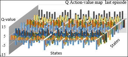
The action-value map at the end of the last episode shows some clear patterns. Most of the rewarding actions transition from a large number of states (X-axis) to a smaller number of states (Y-axis). The chart illustrates the following issues with the small training sample:
- The small size of the training set forces us to use an approximate representation of each feature. The purpose is to increase the odds that most buckets have at least one data point.
- However, a loose function approximation tends to group quite different states into the same bucket.
- The bucket with a very low number can potentially mischaracterize one property or feature of a state.