
9.6 Asymptotic Principal Component Analysis
So far, our discussion of PCA assumes that the number of assets is smaller than the number of time periods, that is, k < T. To deal with situations of a small T and large k, Conner and Korajczyk (1986, 1988) developed the concept of asymptotic principal component analysis (APCA), which is similar to the traditional PCA but relies on the asymptotic results as the number of assets k increases to infinity. Thus, the APCA is based on eigenvalue–eigenvector analysis of the T × T matrix
![]()
where ![]() is the T-dimensional vector of ones and
is the T-dimensional vector of ones and ![]() with
with ![]() being the sample mean of the ith return series. Conner and Korajczyk (1988) showed that as k → ∞ eigenvalue–eigenvector analysis of
being the sample mean of the ith return series. Conner and Korajczyk (1988) showed that as k → ∞ eigenvalue–eigenvector analysis of ![]() is equivalent to the traditional statistical factor analysis. In other words, the APCA estimates of the factors
is equivalent to the traditional statistical factor analysis. In other words, the APCA estimates of the factors ![]() are the first m eigenvectors of
are the first m eigenvectors of ![]() . Let
. Let ![]() be the m × T matrix consisting of the first m eigenvectors of
be the m × T matrix consisting of the first m eigenvectors of ![]() . Then
. Then ![]() is the tth column of
is the tth column of ![]() . Using an idea similar to the estimation of BARRA factor models, Connor and Korajczyk (1988) propose refining the estimation of
. Using an idea similar to the estimation of BARRA factor models, Connor and Korajczyk (1988) propose refining the estimation of ![]() as follows:
as follows:
1. Use the sample covariance matrix ![]() to obtain an initial estimate of
to obtain an initial estimate of ![]() for t = 1, … , T.
for t = 1, … , T.
2. For each asset, perform the OLS estimation of the model
![]()
where ![]() and compute the residual variance
and compute the residual variance ![]() .
.
3. Form the diagonal matrix ![]() and rescale the returns as
and rescale the returns as
![]()
4. Compute the T × T covariance matrix using ![]() as
as
![]()
where ![]() is the k-dimensional vector of the column means of
is the k-dimensional vector of the column means of ![]() , and perform eigenvalue–eigenvector analysis of
, and perform eigenvalue–eigenvector analysis of ![]() to obtain a refined estimate of
to obtain a refined estimate of ![]() .
.
9.6.1 Selecting the Number of Factors
Two methods are available in the literature to help select the number of factors in factor analysis. The first method proposed by Connor and Korajczyk (1993) makes use of the idea that if m is the proper number of common factors, then there should be no significant decrease in the cross-sectional variance of the asset specific error ϵit when the number of factors moves from m to m + 1. The second method proposed by Bai and Ng (2002) adopts some information criteria to select the number of factors. This latter method is based on the observation that the eigenvalue–eigenvector analysis of ![]() solves the least-squares problem
solves the least-squares problem
![]()
Assume that there are m factors so that ![]() is m-dimensional. Let
is m-dimensional. Let ![]() be the residual variance of the inner regression of the prior least-squares problem for asset i. This is done by using
be the residual variance of the inner regression of the prior least-squares problem for asset i. This is done by using ![]() obtained from the APCA analysis. Define the cross-sectional average of the residual variances as
obtained from the APCA analysis. Define the cross-sectional average of the residual variances as
![]()
The criteria proposed by Bai and Ng (2002) are

where M is a prespecified positive integer denoting the maximum number of factors and ![]() . One selects m that minimizes either Cp1(m) or Cp2(m) for 0 ≤ m ≤ M. In practice, the two criteria may select different numbers of factors.
. One selects m that minimizes either Cp1(m) or Cp2(m) for 0 ≤ m ≤ M. In practice, the two criteria may select different numbers of factors.
9.6.2 An Example
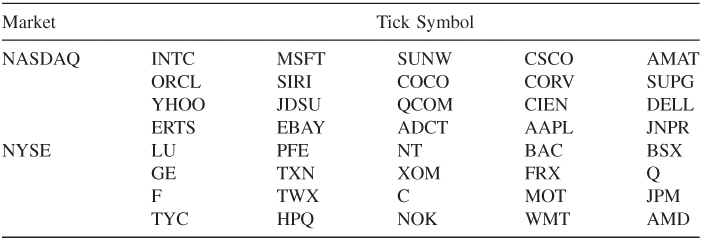
To demonstrate asymptotic principal component analysis, we consider monthly simple returns of 40 stocks from January 2001 to December 2003 for 36 observations. Thus, we have k = 40 and T = 36. The tick symbols of stocks used are given in Table 9.6. These stocks are among those heavily traded on NASDAQ and the NYSE on a particular day of September 2004. The main S-Plus command used is mfactor.
Table 9.6 Tick Symbols of Stocks Used in Asymptotic Principal Component Analysis for Sample Period from January 2001 to December 2003
To select the number of factors, we used the two methods discussed earlier. The Connor–Korajczyk method selects m = 1, whereas the Bai–Ng method uses m = 6. For the latter method, the two criteria provide different results.
> dim(rtn) % rtn is the return data.
[1] 36 40
> nf.ck=mfactor(rtn,k=‘ck’,max.k=10,sig=0.05)
> nf.ck
Call:
mfactor(x = rtn, k = “ck”, max.k = 10, sig = 0.05)
Factor Model:
Factors Variables Periods
1 40 36
Factor Loadings:
Min. 1st Qu. Median Mean 3rd Qu. Max.
F.1 0.069 0.432 0.629 0.688 1.071 1.612
Regression R-squared:
Min. 1st Qu. Median Mean 3rd Qu. Max.
0.090 0.287 0.487 0.456 0.574 0.831
> nf.bn=mfactor(rtn,k=‘bn’,max.k=10,sig=0.05)
Warning messages:
Cp1 and Cp2 did not yield same result. The smaller one
is used.
> nf.bn$k
[1] 6
Using m = 6, we apply APCA to the returns. The scree plot and estimated factor returns can also be obtained.
> apca = mfactor(rtn,k=6)
> apca
Call:
mfactor(x = rtn, k = 6)
Factor Model:
Factors Variables Periods
6 40 36
Factor Loadings:
Min 1st Qu. Median Mean 3rd Qu. Max.
F.1 0.048 0.349 0.561 0.643 0.952 2.222
F.2 -1.737 0.084 0.216 0.214 0.323 1.046
F.3 -1.512 0.002 0.076 0.102 0.255 1.093
F.4 -0.965 -0.035 0.078 0.048 0.202 0.585
F.5 -0.722 -0.008 0.056 0.066 0.214 0.729
F.6 -0.840 -0.088 0.003 0.003 0.071 0.635
Regression R-squared:
Min. 1st Qu. Median Mean 3rd Qu. Max.
0.219 0.480 0.695 0.651 0.801 0.999
> screeplot.mfactor(apca)
> fplot(factors(apca))
Figure 9.7 shows the scree plot of the APCA for the 40 stock returns. The 6 common factors used explain about 89.4% of the variability. Figure 9.8 gives the time plots of the returns of the 6 estimated factors.
Figure 9.7 Scree plot of asymptotic principal component analysis applied to monthly simple returns of 40 stocks. Sample period is from January 2001 to December 2003.

Figure 9.8 Time plots of factor returns derived from applying asymptotic principal component analysis to monthly simple returns of 40 stocks. Sample period is from January 2001 to December 2003.

Exercises
1. Consider the monthly simple excess returns, in percentages and including dividends, of 13 stocks and the S&P 500 composite index from January 1990 to December 2008. The monthly 3-month Treasury bill rate in the secondary market is used as the risk-free interest rate to compute the excess returns. The tick symbols for the stocks are AA, AXP, CAT, DE, F, FDX, HPQ, IBM, JNJ, KMB, MMM, PG, and WFC. The data are in the file m-fac-ex-9008.txt. Perform the market model analysis of Section 9.2.1 for the 13 stock returns to obtain the estimates of βi, ![]() , and R2 for each stock return series.
, and R2 for each stock return series.
2. Consider the monthly log stock returns, in percentages and including dividends, of Merck & Company, Johnson & Johnson, General Electric, General Motors, Ford Motor Company, and value-weighted index from January 1960 to December 2008; see the file m-mrk2vw.txt of Exercise 8.1 of Chapter 8.
a. Perform a principal component analysis of the data using the sample covariance matrix.
b. Perform a principal component analysis of the data using the sample correlation matrix.
c. Perform a statistical factor analysis on the data. Identify the number of common factors. Obtain estimates of factor loadings using both the principal component and maximum-likelihood methods.
3. The file m-excess-c10sp-9003.txt contains the monthly simple excess returns of 10 stocks and the S&P 500 index. The 3-month Treasury bill rate on the secondary market is used to compute the excess returns. The sample period is from January 1990 to December 2003 for 168 observations. The 11 columns in the file contain the returns for ABT, LLY, MRK, PFE, F, GM, BP, CVX, RD, XOM, and SP5, respectively. Analyze the 10 stock excess returns using the single-factor market model. Plot the beta estimate and R2 for each stock, and use the global minimum variance portfolio to compare the covariance matrices of the fitted model and the data.
4. Again, consider the 10 stock returns in m-excess-c10sp-9003.txt. The stocks are from companies in 3 industrial sectors. ABT, LLY, MRK, and PFE are major drug companies, F and GM are automobile companies, and the rest are big oil companies. Analyze the excess returns using the BARRA industrial factor model. Plot the 3-factor realizations and comment on the adequacy of the fitted model.
5. Again, consider the 10 excess stock returns in the file m-excess-c10sp-9003.txt. Perform a principal component analysis on the returns and obtain the scree plot. How many common factors are there? Why? Interpret the common factors.
6. Again, consider the 10 excess stock returns in the file m-excess-c10sp-9003.txt. Perform a statistical factor analysis. How many common factors are there if the 5% significance level is used? Plot the estimated factor loadings of the fitted model. Are the common factors meaningful?
7. The file m-fedip.txt contains year, month, effective federal funds rate, and the industrial production index from July 1954 to December 2003. The industrial production index is seasonally adjusted. Use the federal funds rate and the industrial production index as the macroeconomic variables. Fit a macroeconomic factor model to the 10 excess returns in m-excess-c10sp-9003.txt. You can use a VAR model to obtain the surprise series of the macroeconomic variables. Comment on the fitted factor model.
Alexander, C.(2001). Market Models: A Guide to Financial Data Analysis. Wiley,Hoboken, NJ.
Bai, J. andNg, S.(2002).Determining the number of factors in approximate factor models. Econometrica 70: 191–221.
Campbell, J. Y.,Lo, A. W., andMacKinlay, A. C.(1997). The Econometrics of Financial Markets. Princeton University Press,Princeton, NJ.
Chen, N. F.,Roll, R., andRoss, S. A.(1986).Economic forces and the stock market. Journal of Business 59: 383–404.
Connor, G.(1995).The three types of factor models: A comparison of their explanatory power. Financial Analysts Journal 51: 42–46.
Connor, G. andKorajczyk, R. A.(1986).Performance measurement with the arbitrage pricing theory: A new framework for analysis. Journal of Financial Economics 15: 373–394.
Connor, G. andKorajczyk, R. A.(1988).Risk and return in an equilibrium APT: Application of a new test methodology. Journal of Financial Economics 21: 255–289.
Connor, G. andKorajczyk, R. A.(1993).A test for the number of factors in an approximate factor model. Journal of Finance 48: 1263–1292.
Fama, E. andFrench, K. R.(1992).The cross-section of expected stock returns. Journal of Finance 47: 427–465.
Grinold, R. C. andKahn, R. N.(2000). Active Portfolio Management: A Quantitative Approach for Producing Superior Returns and Controlling Risk, 2nd ed.McGraw-Hill,New York.
Johnson, R. A. andWichern, D. W.(2007). Applied Multivariate Statistical Analysis, 6th ed.Prentice Hall,Upper Saddle River, NJ.
Kaiser, H. F.(1958).The varimax criterion for analytic rotation in factor analysis. Psychometrika 23: 187–200.
Sharpe, W.(1970). Portfolio Theory and Capital Markets. McGraw-Hill,New York.
Zivot, E. andWang, J.(2003). Modeling Financial Time Series with S-Plus. SpringerNew York.