
Besides the return series, we also consider the volatility process and the behavior of extreme returns of an asset. The volatility process is concerned with the evolution of conditional variance of the return over time. This is a topic of interest because, as shown in Figures 1.2 and 1.3, the variabilities of returns vary over time and appear in clusters. In application, volatility plays an important role in pricing options and risk management. By extremes of a return series, we mean the large positive or negative returns. Table 1.2 shows that the minimum and maximum of a return series can be substantial. The negative extreme returns are important in risk management, whereas positive extreme returns are critical to holding a short position. We study properties and applications of extreme returns, such as the frequency of occurrence, the size of an extreme, and the impacts of economic variables on the extremes, in Chapter 7.
Other financial time series considered in the book include interest rates, exchange rates, bond yields, and quarterly earning per share of a company. Figure 1.5 shows the time plots of two U.S. monthly interest rates. They are the 10-year and 1-year Treasury constant maturity rates from April 1954 to February 2009. As expected, the two interest rates moved in unison, but the 1-year rates appear to be more volatile. Figure 1.6 shows the daily exchange rate between the U.S. dollar and the Japanese yen from January 4, 2000, to March 27, 2009. From the plot, the exchange rate encountered occasional big changes in the sampling period. Table 1.3 provides some descriptive statistics for selected U.S. financial time series. The monthly bond returns obtained from CRSP are Fama bond portfolio returns from January 1952 to December 2008. The interest rates are obtained from the Federal Reserve Bank of St. Louis. The weekly 3-month Treasury bill rate started on January 8, 1954, and the 6-month rate started on December 12, 1958. Both series ended on March 27, 2009. For the interest rate series, the sample means are proportional to the time to maturity, but the sample standard deviations are inversely proportional to the time to maturity. For the bond returns, the sample standard deviations are positively related to the time to maturity, whereas the sample means remain stable for all maturities. Most of the series considered have positive excess kurtoses.
Figure 1.5 Time plots of monthly U.S. interest rates from April 1953 to February 2009: (a) 10-year Treasury constant maturity rate and (b) 1-year maturity rate.
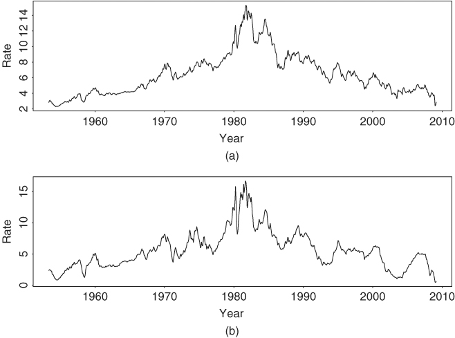
Table 1.3 Descriptive Statistics of Selected U.S. Financial Time Seriesa

aThe data are in percentages. The weekly 3-month Treasury bill rate started from January 8, 1954, and the 6-month rate started from December 12, 1958. The sample sizes for Treasury bill rates are 2882 and 2625, respectively. Data sources are given in the text.
With respect to the empirical characteristics of returns shown in Table 1.2, Chapters 2–4 focus on the first four moments of a return series and Chapter 7 on the behavior of minimum and maximum returns. Chapters 8 and 10 are concerned with moments of and the relationships between multiple asset returns, and Chapter 5 addresses properties of asset returns when the time interval is small. An introduction to mathematical finance is given in Chapter 6.