1.2 Distributional Properties of Returns

To study asset returns, it is best to begin with their distributional properties. The objective here is to understand the behavior of the returns across assets and over time. Consider a collection of N assets held for T time periods, say, t = 1, …, T. For each asset i, let rit be its log return at time t. The log returns under study are {rit;i = 1, …, N;t = 1, …, T}. One can also consider the simple returns {Rit;i = 1, …, N;t = 1, …, T} and the log excess returns {zit;i = 1, …, N;t = 1, …, T}.

1.2.1 Review of Statistical Distributions and Their Moments

We briefly review some basic properties of statistical distributions and the moment equations of a random variable. Let Rk be the k-dimensional Euclidean space. A point in Rk is denoted by x ∈ Rk. Consider two random vectors X = (X1, …, Xk)′ and Y = (Y1, …, Yq)′. Let P(X ∈ A, Y ∈ B) be the probability that X is in the subspace A ⊂ Rk and Y is in the subspace B ⊂ Rq. For most of the cases considered in this book, both random vectors are assumed to be continuous.

Joint Distribution

The function

where x ∈ Rp, y ∈ Rq, and the inequality ≤ is a component-by-component operation, is a joint distribution function of X and Y with parameter θ. Behavior of X and Y is characterized by FX, Y(x, y;θ). If the joint probability density function fx, y(x, y;θ) of X and Y exists, then

In this case, X and Y are continuous random vectors.

Marginal Distribution

The marginal distribution of X is given by

Thus, the marginal distribution of X is obtained by integrating out Y. A similar definition applies to the marginal distribution of Y.

If k = 1, X is a scalar random variable and the distribution function becomes

which is known as the cumulative distribution function (CDF) of X. The CDF of a random variable is nondecreasing [i.e., FX(x1) ≤ FX(x2) if x1 ≤ x2] and satisfies FX(− ∞) = 0 and FX(∞) = 1. For a given probability p, the smallest real number xp such that p ≤ FX(xp) is called the 100pth quantile of the random variable X. More specifically,

We use the CDF to compute the p value of a test statistic in the book.

Conditional Distribution

The conditional distribution of X given Y ≤ y is given by

If the probability density functions involved exist, then the conditional density of X given Y = y is

1.8

where the marginal density function fy(y;θ) is obtained by

From Eq. (1.8), the relation among joint, marginal, and conditional distributions is

1.9

This identity is used extensively in time series analysis (e.g., in maximum-likelihood estimation). Finally, X and Y are independent random vectors if and only if fx|y(x;θ) = fx(x;θ). In this case, fx, y(x, y;θ) = fx(x;θ)fy(y;θ).

Moments of a Random Variable

The ℓth moment of a continuous random variable X is defined as

where E stands for expectation and f(x) is the probability density function of X. The first moment is called the mean or expectation of X. It measures the central location of the distribution. We denote the mean of X by μx. The ℓth central moment of X is defined as

provided that the integral exists. The second central moment, denoted by , measures the variability of X and is called the variance of X. The positive square root, σx, of variance is the standard deviation of X. The first two moments of a random variable uniquely determine a normal distribution. For other distributions, higher order moments are also of interest.

The third central moment measures the symmetry of X with respect to its mean, whereas the fourth central moment measures the tail behavior of X. In statistics, skewness and kurtosis, which are normalized third and fourth central moments of X, are often used to summarize the extent of asymmetry and tail thickness. Specifically, the skewness and kurtosis of X are defined as

The quantity K(x) − 3 is called the excess kurtosis because K(x) = 3 for a normal distribution. Thus, the excess kurtosis of a normal random variable is zero. A distribution with positive excess kurtosis is said to have heavy tails, implying that the distribution puts more mass on the tails of its support than a normal distribution does. In practice, this means that a random sample from such a distribution tends to contain more extreme values. Such a distribution is said to be leptokurtic. On the other hand, a distribution with negative excess kurtosis has short tails (e.g., a uniform distribution over a finite interval). Such a distribution is said to be platykurtic.

In application, skewness and kurtosis can be estimated by their sample counterparts. Let {x1, …, xT} be a random sample of X with T observations. The sample mean is

1.10

the sample variance is

1.11

the sample skewness is

1.12

and the sample kurtosis is

1.13

Under the normality assumption, (x) and are distributed asymptotically as normal with zero mean and variances 6/T and 24/T, respectively; see Snedecor and Cochran (1980, p. 78). These asymptotic properties can be used to test the normality of asset returns. Given an asset return series {r1, …, rT}, to test the skewness of the returns, we consider the null hypothesis H0 : S(r) = 0 versus the alternative hypothesis Ha : S(r) ≠ 0. The t-ratio statistic of the sample skewness in Eq. (1.12) is

The decision rule is as follows. Reject the null hypothesis at the α significance level, if |t| > Zα/2, where Zα/2 is the upper 100(α/2)th quantile of the standard normal distribution. Alternatively, one can compute the p value of the test statistic t and reject H0 if and only if the p value is less than α.

Similarly, one can test the excess kurtosis of the return series using the hypotheses H0 : K(r) − 3 = 0 versus Ha : K(r) − 3 ≠ 0. The test statistic is

which is asymptotically a standard normal random variable. The decision rule is to reject H0 if and only if the p value of the test statistic is less than the significance level α. Jarque and Bera (1987) (JB) combine the two prior tests and use the test statistic

which is asymptotically distributed as a chi-squared random variable with 2 degrees of freedom, to test for the normality of rt. One rejects H0 of normality if the p value of the JB statistic is less than the significance level.

Table 1.2 Descriptive Statistics for Daily and Monthly Simple and Log Returns of Selected Indexes and Stocks2

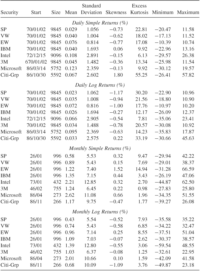
a Returns are in percentages and the sample period ends on December 31, 2008. The statistics are defined in eqs. (1.10)–(1.13), and VW, EW and SP denote value-weighted, equal-weighted, and S&P composite index.

R Demonstration

In the following program code > is the prompt character and % denotes explanation:

S-Plus Demonstration

In the following program code > is the prompt character and % marks explanation:

1.2.2 Distributions of Returns

The most general model for the log returns {rit ; i = 1, …, N ; t = 1, …, T} is its joint distribution function:

1.14

where Y is a state vector consisting of variables that summarize the environment in which asset returns are determined and θ is a vector of parameters that uniquely determines the distribution function Fr(·). The probability distribution Fr(·) governs the stochastic behavior of the returns rit and Y. In many financial studies, the state vector Y is treated as given and the main concern is the conditional distribution of {rit} given Y. Empirical analysis of asset returns is then to estimate the unknown parameter θ and to draw statistical inference about the behavior of {rit} given some past log returns.

The model in Eq. (1.14) is too general to be of practical value. However, it provides a general framework with respect to which an econometric model for asset returns rit can be put in a proper perspective.

Some financial theories such as the capital asset pricing model (CAPM) of Sharpe (1964) focus on the joint distribution of N returns at a single time index t (i.e., the distribution of {r1t, …, rNt}). Other theories emphasize the dynamic structure of individual asset returns (i.e., the distribution of {ri1, …, riT} for a given asset i). In this book, we focus on both. In the univariate analysis of Chapters 2–7, our main concern is the joint distribution of for asset i. To this end, it is useful to partition the joint distribution as

1.15

where, for simplicity, the parameter θ is omitted. This partition highlights the temporal dependencies of the log return rit. The main issue then is the specification of the conditional distribution F(rit|ri, t−1, ·), in particular, how the conditional distribution evolves over time. In finance, different distributional specifications lead to different theories. For instance, one version of the random-walk hypothesis is that the conditional distribution F(rit|ri, t−1, …, ri1) is equal to the marginal distribution F(rit). In this case, returns are temporally independent and, hence, not predictable.

It is customary to treat asset returns as continuous random variables, especially for index returns or stock returns calculated at a low frequency, and use their probability density functions. In this case, using the identity in Eq. (1.9), we can write the partition in Eq. (1.15) as

1.16

For high-frequency asset returns, discreteness becomes an issue. For example, stock prices change in multiples of a tick size on the New York Stock Exchange (NYSE). The tick size was of a dollar before July 1997 and was of a dollar from July 1997 to January 2001. Therefore, the tick-by-tick return of an individual stock listed on the NYSE is not continuous. We discuss high-frequency stock price changes and time durations between price changes later in Chapter 5.

Equation (1.16) suggests that conditional distributions are more relevant than marginal distributions in studying asset returns. However, the marginal distributions may still be of some interest. In particular, it is easier to estimate marginal distributions than conditional distributions using past returns. In addition, in some cases, asset returns have weak empirical serial correlations, and, hence, their marginal distributions are close to their conditional distributions.

Several statistical distributions have been proposed in the literature for the marginal distributions of asset returns, including normal distribution, lognormal distribution, stable distribution, and scale mixture of normal distributions. We briefly discuss these distributions.

Normal Distribution

A traditional assumption made in financial study is that the simple returns {Rit|t = 1, …, T} are independently and identically distributed as normal with fixed mean and variance. This assumption makes statistical properties of asset returns tractable. But it encounters several difficulties. First, the lower bound of a simple return is − 1. Yet the normal distribution may assume any value in the real line and, hence, has no lower bound. Second, if Rit is normally distributed, then the multiperiod simple return Rit[k] is not normally distributed because it is a product of one-period returns. Third, the normality assumption is not supported by many empirical asset returns, which tend to have a positive excess kurtosis.

Lognormal Distribution

Another commonly used assumption is that the log returns rt of an asset are independent and identically distributed (iid) as normal with mean μ and variance σ2. The simple returns are then iid lognormal random variables with mean and variance given by

1.17

These two equations are useful in studying asset returns (e.g., in forecasting using models built for log returns). Alternatively, let m1 and m2 be the mean and variance of the simple return Rt, which is lognormally distributed. Then the mean and variance of the corresponding log return rt are

Because the sum of a finite number of iid normal random variables is normal, rt[k] is also normally distributed under the normal assumption for {rt}. In addition, there is no lower bound for rt, and the lower bound for Rt is satisfied using 1 + Rt = exp(rt). However, the lognormal assumption is not consistent with all the properties of historical stock returns. In particular, many stock returns exhibit a positive excess kurtosis.

Stable Distribution

The stable distributions are a natural generalization of normal in that they are stable under addition, which meets the need of continuously compounded returns rt. Furthermore, stable distributions are capable of capturing excess kurtosis shown by historical stock returns. However, nonnormal stable distributions do not have a finite variance, which is in conflict with most finance theories. In addition, statistical modeling using nonnormal stable distributions is difficult. An example of nonnormal stable distributions is the Cauchy distribution, which is symmetric with respect to its median but has infinite variance.

Scale Mixture of Normal Distributions

Recent studies of stock returns tend to use scale mixture or finite mixture of normal distributions. Under the assumption of scale mixture of normal distributions, the log return rt is normally distributed with mean μ and variance σ2 [i.e., rt ∼ N(μ, σ2)]. However, σ2 is a random variable that follows a positive distribution (e.g., σ−2 follows a gamma distribution). An example of finite mixture of normal distributions is

where X is a Bernoulli random variable such that P(X = 1) = α and P(X = 0) = 1 − α with 0 < α < 1, is small, and is relatively large. For instance, with α = 0.05, the finite mixture says that 95% of the returns follow and 5% follow . The large value of enables the mixture to put more mass at the tails of its distribution. The low percentage of returns that are from says that the majority of the returns follow a simple normal distribution. Advantages of mixtures of normal include that they maintain the tractability of normal, have finite higher order moments, and can capture the excess kurtosis. Yet it is hard to estimate the mixture parameters (e.g., the α in the finite-mixture case).

Figure 1.1 shows the probability density functions of a finite mixture of normal, Cauchy, and standard normal random variable. The finite mixture of normal is (1 − X)N(0, 1) + X × N(0, 16) with X being Bernoulli such that P(X = 1) = 0.05, and the density function of Cauchy is

It is seen that the Cauchy distribution has fatter tails than the finite mixture of normal, which, in turn, has fatter tails than the standard normal.

1.2.3 Multivariate Returns

Let rt = (r1t, …, rNt)′ be the log returns of N assets at time t. The multivariate analyses of Chapters 8 and 10 are concerned with the joint distribution of . This joint distribution can be partitioned in the same way as that of Eq. (1.15). The analysis is then focused on the specification of the conditional distribution function F(rt|rt−1, …, r1, θ). In particular, how the conditional expectation and conditional covariance matrix of rt evolve over time constitute the main subjects of Chapters 8 and 10.

The mean vector and covariance matrix of a random vector X = (X1, …, Xp) are defined as

provided that the expectations involved exist. When the data {x1, …, xT} of X are available, the sample mean and covariance matrix are defined as

These sample statistics are consistent estimates of their theoretical counterparts provided that the covariance matrix of X exists. In the finance literature, multivariate normal distribution is often used for the log return rt.

1.2.4 Likelihood Function of Returns

The partition of Eq. (1.15) can be used to obtain the likelihood function of the log returns {r1, …, rT} of an asset, where for ease in notation the subscript i is omitted from the log return. If the conditional distribution f(rt|rt−1, …, r1, θ) is normal with mean μt and variance , then θ consists of the parameters in μt and , and the likelihood function of the data is

1.18

where f(r1;θ) is the marginal density function of the first observation r1. The value of θ that maximizes this likelihood function is the maximum-likelihood estimate (MLE) of θ. Since the log function is monotone, the MLE can be obtained by maximizing the log-likelihood function,

which is easier to handle in practice. The log-likelihood function of the data can be obtained in a similar manner if the conditional distribution f(rt|rt−1, …, r1;θ) is not normal.

1.2.5 Empirical Properties of Returns

The data used in this section are obtained from the Center for Research in Security Prices (CRSP) of the University of Chicago. Dividend payments, if any, are included in the returns. Figure 1.2 shows the time plots of monthly simple returns and log returns of IBM stock from January 1926 to December 2008. A time plot shows the data against the time index. The upper plot is for the simple returns. Figure 1.3 shows the same plots for the monthly returns of value-weighted market index. As expected, the plots show that the basic patterns of simple and log returns are similar.

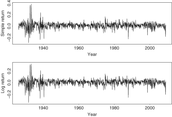
Table 1.2 provides some descriptive statistics of simple and log returns for selected U.S. market indexes and individual stocks. The returns are for daily and monthly sample intervals and are in percentages. The data spans and sample sizes are also given in Table 1.2. From the table, we make the following observations. (a) Daily returns of the market indexes and individual stocks tend to have high excess kurtoses. For monthly series, the returns of market indexes have higher excess kurtoses than individual stocks. (b) The mean of a daily return series is close to zero, whereas that of a monthly return series is slightly larger. (c) Monthly returns have higher standard deviations than daily returns. (d) Among the daily returns, market indexes have smaller standard deviations than individual stocks. This is in agreement with common sense. (e) The skewness is not a serious problem for both daily and monthly returns. (f) The descriptive statistics show that the difference between simple and log returns is not substantial.

Figure 1.4 shows the empirical density functions of monthly simple and log returns of IBM stock from 1926 to 2008. Also shown, by a dashed line, in each graph is the normal probability density function evaluated by using the sample mean and standard deviation of IBM returns given in Table 1.2. The plots indicate that the normality assumption is questionable for monthly IBM stock returns. The empirical density function has a higher peak around its mean, but fatter tails than that of the corresponding normal distribution. In other words, the empirical density function is taller and skinnier, but with a wider support than the corresponding normal density.