
10.4 GARCH Models for Bivariate Returns
Since the same techniques can be used to generalize many univariate volatility models to the multivariate case, we focus our discussion on the multivariate GARCH model. Other multivariate volatility models can also be used.
For a k-dimensional return series ![]() , a multivariate GARCH model uses “exact equations” to describe the evolution of the k(k + 1)/2-dimensional vector
, a multivariate GARCH model uses “exact equations” to describe the evolution of the k(k + 1)/2-dimensional vector ![]() over time. By exact equation, we mean that the equation does not contain any stochastic shock. However, the exact equation may become complicated even in the simplest case of k = 2 for which
over time. By exact equation, we mean that the equation does not contain any stochastic shock. However, the exact equation may become complicated even in the simplest case of k = 2 for which ![]() is three dimensional. To keep the model simple, some restrictions are often imposed on the equations.
is three dimensional. To keep the model simple, some restrictions are often imposed on the equations.
10.4.1 Constant-Correlation Models
To keep the number of volatility equations low, Bollerslev (1990) considers the special case in which the correlation coefficient ρ21, t = ρ21 is time invariant, where |ρ21| < 1. Under such an assumption, ρ21 is a constant parameter and the volatility model consists of two equations for ![]() , which is defined as
, which is defined as ![]() . A GARCH(1,1) model for
. A GARCH(1,1) model for ![]() becomes
becomes
10.21 ![]()
where ![]() ,
, ![]() is a two-dimensional positive vector, and
is a two-dimensional positive vector, and ![]() and
and ![]() are 2 × 2 nonnegative definite matrices. More specifically, the model can be expressed in detail as
are 2 × 2 nonnegative definite matrices. More specifically, the model can be expressed in detail as
10.22 ![]()
where αi0 > 0 for i = 1 and 2. Defining ![]() , we can rewrite the prior model as
, we can rewrite the prior model as
![]()
which is a bivariate ARMA(1,1) model for the ![]() process. This result is a direct generalization of the univariate GARCH(1,1) model of Chapter 3. Consequently, some properties of model (10.22) are readily available from those of the bivariate ARMA(1,1) model of Chapter 8. In particular, we have the following results:
process. This result is a direct generalization of the univariate GARCH(1,1) model of Chapter 3. Consequently, some properties of model (10.22) are readily available from those of the bivariate ARMA(1,1) model of Chapter 8. In particular, we have the following results:
1. If all of the eigenvalues of ![]() are positive, but less than 1, then the bivariate ARMA(1,1) model for
are positive, but less than 1, then the bivariate ARMA(1,1) model for ![]() is weakly stationary and, hence,
is weakly stationary and, hence, ![]() exists. This implies that the shock process
exists. This implies that the shock process ![]() of the returns has a positive-definite unconditional covariance matrix. The unconditional variances of the elements of
of the returns has a positive-definite unconditional covariance matrix. The unconditional variances of the elements of ![]() are
are ![]() , and the unconditional covariance between a1t and a2t is ρ21σ1σ2.
, and the unconditional covariance between a1t and a2t is ρ21σ1σ2.
2. If α12 = β12 = 0, then the volatility of a1t does not depend on the past volatility of a2t. Similarly, if α21 = β21 = 0, then the volatility of a2t does not depend on the past volatility of a1t.
3. If both ![]() and
and ![]() are diagonal, then the model reduces to two univariate GARCH(1,1) models. In this case, the two volatility processes are not dynamically related.
are diagonal, then the model reduces to two univariate GARCH(1,1) models. In this case, the two volatility processes are not dynamically related.
4. Volatility forecasts of the model can be obtained by using forecasting methods similar to those of a vector ARMA(1,1) model; see the univariate case in Chapter 3. The 1-step-ahead volatility forecast at the forecast origin h is
![]()
For the ℓ-step-ahead forecast, we have
![]()
These forecasts are for the marginal volatilities of ait. The ℓ-step-ahead forecast of the covariance between a1t and a2t is ![]() , where
, where ![]() is the estimate of ρ21 and σii, h(ℓ) are the elements of
is the estimate of ρ21 and σii, h(ℓ) are the elements of ![]() .
.
Example 10.4
Again, consider the daily log returns of Hong Kong and Japanese markets of Example 10.1. Using a bivariate GARCH model, we obtain a constant correlation model that fits the data reasonably well. The mean equations of the bivariate model are
![]()
where the standard errors of the two estimates are 0.050 and 0.048, respectively. The volatility equations are

where the numbers in parentheses are standard errors. The estimated constant correlation between the two returns is 0.668.
Let ![]() be the standardized residuals, where
be the standardized residuals, where ![]() . The Ljung–Box statistics of
. The Ljung–Box statistics of ![]() give Q2(4) = 17.29(0.37) and Q2(12) = 48.21(0.46), where the number in parentheses denotes the p value. Here the p values are based on chi-squared distributions with 16 and 48 degrees of freedom, respectively. The Q statistics of individual series ãit shown in S-Plus output also fail to indicate any model inadequancy. Consequently, the constant correlation model in Eq. (10.23) fits the data reasonably well. Figure 10.7 shows the fitted volatility processes of model (10.23), which can be compared with those of Example 10.1.
give Q2(4) = 17.29(0.37) and Q2(12) = 48.21(0.46), where the number in parentheses denotes the p value. Here the p values are based on chi-squared distributions with 16 and 48 degrees of freedom, respectively. The Q statistics of individual series ãit shown in S-Plus output also fail to indicate any model inadequancy. Consequently, the constant correlation model in Eq. (10.23) fits the data reasonably well. Figure 10.7 shows the fitted volatility processes of model (10.23), which can be compared with those of Example 10.1.
Figure 10.7 Estimated volatilities for daily log returns in percentages of stock market indexes for Hong Kong and Japan from January 4, 2006, to December 30, 2008: (a) Hong Kong market and (b) Japanese market. Model used is Eq. (10.23).
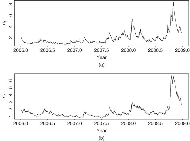
The model in Eq. (10.23) shows two uncoupled volatility equations, indicating that the volatilities of the two markets are not dynamically related, but they are contemporaneously correlated. We refer to the model as a bivariate diagonal constant-correlation model. In practice, this type of models might not be suitable because there exists the possibility of dynamic dependence in volatility among markets, that is, the spillover effect in volatility. Finally, the constant-correlation model can easily be estimated using S-Plus:
> mccc = mgarch(rtn∼1,∼ccc(1,1),trace=F)
> summary(mccc)
Example 10.5
As a second illustration, consider the monthly log returns, in percentages, of IBM stock and the S&P 500 index from January 1926 to December 1999 used in Chapter 8. Let r1t and r2t be the monthly log returns for IBM stock and the S&P 500 index, respectively. If a constant-correlation GARCH(1,1) model is entertained, we obtain the mean equations
![]()
where standard errors of the parameters in the first equation are 0.225, 0.029, 0.034, and 0.044, respectively, and the standard error of the parameter in the second equation is 0.155. The volatility equations are

where the numbers in parentheses are standard errors. The constant correlation coefficient is 0.614 with standard error 0.020. Using the standardized residuals, we obtain the Ljung–Box statistics Q2(4) = 16.77(0.21) and Q2(8) = 32.40(0.30), where the p values shown in parentheses are obtained from chi-squared distributions with 13 and 29 degrees of freedom, respectively. Here the degrees of freedom have been adjusted because the mean equations contain three lagged predictors. For the squared standardized residuals, we have ![]() and
and ![]() . Therefore, at the 5% significance level, the standardized residuals
. Therefore, at the 5% significance level, the standardized residuals ![]() have no serial correlations or conditional heteroscedasticities. This bivariate GARCH(1,1) model shows a feedback relationship between the volatilities of the two monthly log returns.
have no serial correlations or conditional heteroscedasticities. This bivariate GARCH(1,1) model shows a feedback relationship between the volatilities of the two monthly log returns.
10.4.2 Time-Varying Correlation Models
A major drawback of the constant-correlation volatility models is that the correlation coefficient tends to change over time in a real application. Consider the monthly log returns of IBM stock and the S&P 500 index used in Example 10.5. It is hard to justify that the S&P 500 index return, which is a weighted average, can maintain a constant-correlation coefficient with IBM return over the past 70 years. Figure 10.8 shows the sample correlation coefficient between the two monthly log return series using a moving window of 120 observations (i.e., 10 years). The correlation changes over time and appears to be decreasing in recent years. The decreasing trend in correlation is not surprising because the ranking of IBM market capitalization among large U.S. industrial companies has changed in recent years. A Lagrange multiplier statistic was proposed recently by Tse (2000) to test constant-correlation coefficients in a multivariate GARCH model.
Figure 10.8 Sample correlation coefficient between monthly log returns of IBM stock and S&P 500 index. Correlation is computed by a moving window of 120 observations. Sample period is from January 1926 to December 1999.
A simple way to relax the constant-correlation constraint within the GARCH framework is to specify an exact equation for the conditional correlation coefficient. This can be done by two methods using the two reparameterizations of ![]() discussed in Section 10.3. First, we use the correlation coefficient directly. Because the correlation coefficient between the returns of IBM stock and S&P 500 index is positive and must be in the interval [0, 1], we employ the equation
discussed in Section 10.3. First, we use the correlation coefficient directly. Because the correlation coefficient between the returns of IBM stock and S&P 500 index is positive and must be in the interval [0, 1], we employ the equation
where
![]()
where σii, t−1 is the conditional variance of the shock ai, t−1. We refer to this equation as a GARCH(1,1) model for the correlation coefficient because it uses the lag-1 cross correlation and the lag-1 cross product of the two shocks. If ![]() , then model (10.25) reduces to the case of constant correlation.
, then model (10.25) reduces to the case of constant correlation.
In summary, a time-varying correlation bivariate GARCH(1,1) model consists of two sets of equations. The first set of equations consists of a bivariate GARCH(1,1) model for the conditional variances, and the second set of equation is a GARCH(1,1) model for the correlation in Eq. (10.25). In practice, a negative sign can be added to Eq. (10.25) if the correlation coefficient is negative. In general, when the sign of correlation is unknown, we can use the Fisher transformation for correlation
![]()
and employ a GARCH model for qt to model the time-varying correlation between two returns.
Example 10.5 (Continued)
Augmenting Eq. (10.25) to the GARCH(1,1) model in Eq. (10.24) for the monthly log returns of IBM stock and the S&P 500 index and performing a joint estimation, we obtain the following model for the two series:
![]()
where standard errors of the three parameters in the first equation are 0.215, 0.026, and 0.034, respectively, and standard error of the parameter in the second equation is 0.151. The volatility equations are

where, as before, standard errors are in parentheses. The conditional correlation equation is
where standard errors of the estimates are 0.050, 0.090, and 0.019, respectively. The parameters of the prior correlation equation are highly significant. Applying the Ljung–Box statistics to the standardized residuals ![]() , we have Q2(4) = 20.57(0.11) and Q2(8) = 36.08(0.21). For the squared standardized residuals, we have
, we have Q2(4) = 20.57(0.11) and Q2(8) = 36.08(0.21). For the squared standardized residuals, we have ![]() and
and ![]() . Therefore, the standardized residuals of the model have no significant serial correlations or conditional heteroscedasticities.
. Therefore, the standardized residuals of the model have no significant serial correlations or conditional heteroscedasticities.
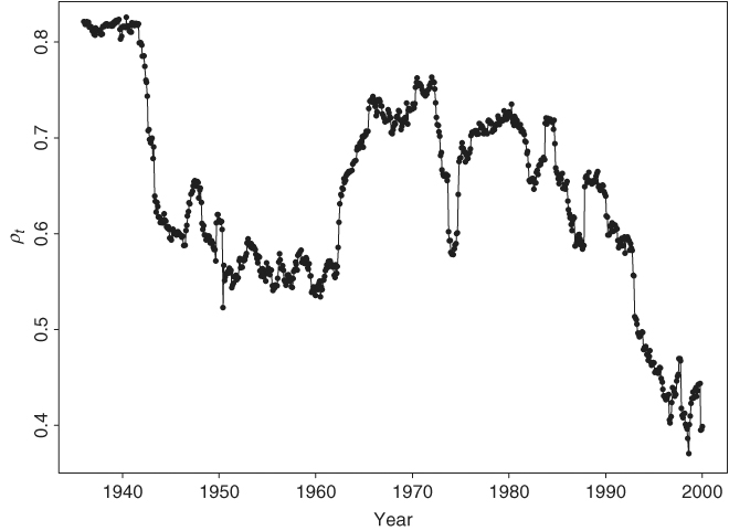
It is interesting to compare this time-varying correlation GARCH(1,1) model with the constant-correlation GARCH(1,1) model in Eq. (10.24). First, the mean and volatility equations of the two models are close. Second, Figure 10.9 shows the fitted conditional correlation coefficient between the monthly log returns of IBM stock and the S&P 500 index based on model (10.27). The plot shows that the correlation coefficient fluctuated over time and became smaller in recent years. This latter characteristic is in agreement with that of Figure 10.8. Third, the average of the fitted correlation coefficients is 0.612, which is essentially the estimate 0.614 of the constant-correlation model in Eq. (10.24). Fourth, using the sample variances of rit as the starting values for the conditional variances and the observations from t = 4 to t = 888, the maximized log-likelihood function is − 3691.21 for the constant-correlation GARCH(1,1) model and − 3679.64 for the time-varying correlation GARCH(1,1) model. Thus, the time-varying correlation model shows some significant improvement over the constant-correlation model. Finally, consider the 1-step-ahead volatility forecasts of the two models at the forecast origin h = 888. For the constant-correlation model in Eq. (10.24), we have a1, 888 = 3.075, a2, 888 = 4.931, σ11, 888 = 77.91, and σ22, 888 = 21.19. Therefore, the 1-step-ahead forecast for the conditional covariance matrix is
![]()
where the covariance is obtained by using the constant-correlation coefficient 0.614. For the time-varying correlation model in Eqs. (10.26) and (10.27), we have a1, 888 = 3.287, a2, 888 = 4.950, σ11, 888 = 83.35, σ22, 888 = 28.56, and ρ888 = 0.546. The 1-step-ahead forecast for the covariance matrix is
![]()
where the forecast of the correlation coefficient is 0.545.
Figure 10.9 Fitted conditional correlation coefficient between monthly log returns of IBM stock and S&P 500 index using time-varying correlation GARCH(1,1) model of Example 10.5. Horizontal line denotes average of 0.612 of correlation coefficients. 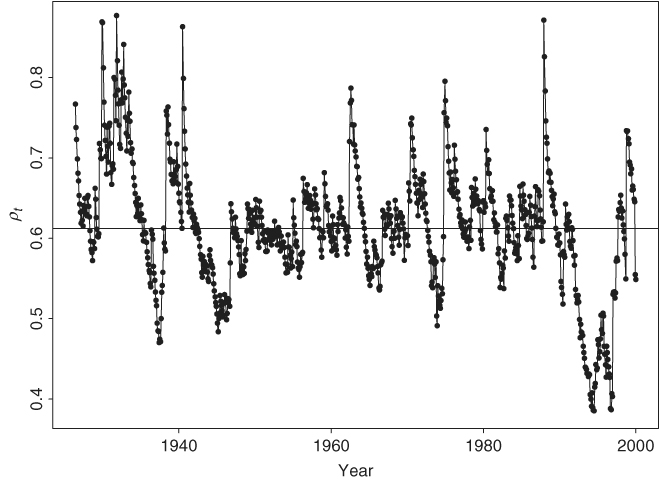
In the second method, we use the Cholesky decomposition of ![]() to model time-varying correlations. For the bivariate case, the parameter vector is
to model time-varying correlations. For the bivariate case, the parameter vector is ![]() ; see Eq. (10.18). A simple GARCH(1,1) type model for
; see Eq. (10.18). A simple GARCH(1,1) type model for ![]() is
is

where b1t = a1t and b2t = a2t − q21, ta1t. Thus, b1t assumes a univariate GARCH(1,1) model, b2t uses a bivariate GARCH(1,1) model, and q21, t is autocorrelated and uses a2, t−1 as an additional explanatory variable. The probability density function relevant to maximum-likelihood estimation is given in Eq. (10.20) with k = 2.
Example 10.5 (Continued)
Again we use the monthly log returns of IBM stock and the S&P 500 index to demonstrate the volatility model in Eq. (10.28). Using the same specification as before, we obtain the fitted mean equations as
![]()
where standard errors of the parameters in the first equation are 0.219, 0.027, and 0.032, respectively, and the standard error of the parameter in the second equation is 0.154. These two mean equations are close to what we obtained before. The fitted volatility model is
where b1t = a1t, and b2t = a2t − q21, tb1t. Standard errors of the parameters in the equation of g11, t are 1.033, 0.022, and 0.037, respectively; those of the parameters in the equation of q21, t are 0.001, 0.002, and 0.0004; and those of the parameters in the equation of g22, t are 0.344, 0.007, 0.013, and 0.015, respectively. All estimates are statistically significant at the 1% level.
The conditional covariance matrix ![]() can be obtained from model (10.29) by using the Cholesky decomposition in Eq. (10.12). For the bivariate case, the relationship is given specifically in Eq. (10.13). Consequently, we obtain the time-varying correlation coefficient as
can be obtained from model (10.29) by using the Cholesky decomposition in Eq. (10.12). For the bivariate case, the relationship is given specifically in Eq. (10.13). Consequently, we obtain the time-varying correlation coefficient as
Using the fitted values of σ11, t and σ22, t, we can compute the standardized residuals to perform model checking. The Ljung–Box statistics for the standardized residuals of model (10.29) give Q2(4) = 19.77(0.14) and Q2(8) = 34.22(0.27). For the squared standardized residuals, we have ![]() and
and ![]() . Thus, the fitted model is adequate in describing the conditional mean and volatility. The model shows a strong dynamic dependence in the correlation; see the coefficient 0.9915 in Eq. (10.29).
. Thus, the fitted model is adequate in describing the conditional mean and volatility. The model shows a strong dynamic dependence in the correlation; see the coefficient 0.9915 in Eq. (10.29).
Figure 10.10 shows the fitted time-varying correlation coefficient in Eq. (10.30). It shows a smoother correlation pattern than that of Figure 10.9 and confirms the decreasing trend of the correlation coefficient. In particular, the fitted correlation coefficients in recent years are smaller than those of the other models. The two time-varying correlation models for the monthly log returns of IBM stock and the S&P 500 index have comparable maximized-likelihood functions of about − 3672, indicating the fits are similar. However, the approach based on the Cholesky decomposition may have some advantages. First, it does not require any parameter constraint in estimation to ensure the positive definiteness of ![]() . If one also uses log transformation for gii, t, then no constraints are needed for the entire volatility model. Second, the log-likelihood function becomes simple under the transformation. Third, the time-varying parameters qij, t and gii, t have nice interpretations. However, the transformation makes inference a bit more complicated because the fitted model may depend on the ordering of elements in
. If one also uses log transformation for gii, t, then no constraints are needed for the entire volatility model. Second, the log-likelihood function becomes simple under the transformation. Third, the time-varying parameters qij, t and gii, t have nice interpretations. However, the transformation makes inference a bit more complicated because the fitted model may depend on the ordering of elements in ![]() ; recall that a1t is not transformed. In theory, the ordering of elements in
; recall that a1t is not transformed. In theory, the ordering of elements in ![]() should have no impact on volatility.
should have no impact on volatility.
Figure 10.10 Fitted conditional correlation coefficient between monthly log returns of IBM stock and S&P 500 index using time-varying correlation GARCH(1,1) model of Example 10.5 with Cholesky decomposition. Horizontal line denotes average of 0.612 of the estimated coefficients.

Finally, the 1-step-ahead forecast of the conditional covariance matrix at the forecast origin t = 888 for the new time-varying correlation model is
![]()
The correlation coefficient of the prior forecast is 0.203, which is substantially smaller than those of the previous two models. However, forecasts of the conditional variances are similar as before.
10.4.3 Dynamic Correlation Models
Using the parameterization in Eq. (10.7), several authors have proposed parsimonious models for ![]() to describe the time-varying correlations. We refer to those models as the dynamic conditional correlation (DCC) models.
to describe the time-varying correlations. We refer to those models as the dynamic conditional correlation (DCC) models.
For k-dimensional returns, Tse and Tsui (2002) assume that the conditional correlation matrix ![]() follows the model
follows the model
![]()
where θ1 and θ2 are scalar parameters, ![]() is a k × k positive-definite matrix with unit diagonal elements, and
is a k × k positive-definite matrix with unit diagonal elements, and ![]() is the k × k sample correlation matrix using shocks from t − m, … , t − 1 for a prespecified m. Typically, one assumes that 0 ≤ θi < 1 and θ1 + θ2 < 1 so that the resulting correlation matrix
is the k × k sample correlation matrix using shocks from t − m, … , t − 1 for a prespecified m. Typically, one assumes that 0 ≤ θi < 1 and θ1 + θ2 < 1 so that the resulting correlation matrix ![]() is positive definite for all t. For a given
is positive definite for all t. For a given ![]() , the model is parsimonious. In applications, the choice of
, the model is parsimonious. In applications, the choice of ![]() and m deserves a careful investigation. One possibility is to let
and m deserves a careful investigation. One possibility is to let ![]() be the sample correlation matrix of the returns. The correlation equation then only employs two parameters.
be the sample correlation matrix of the returns. The correlation equation then only employs two parameters.
Engle (2002) proposes the model
![]()
where ![]() is a positive-definite matrix,
is a positive-definite matrix, ![]() , and
, and ![]() satisfies
satisfies
![]()
where ![]() is the standardized innovation vector with elements
is the standardized innovation vector with elements ![]() ,
, ![]() is the unconditional covariance matrix of
is the unconditional covariance matrix of ![]() , and θ1 and θ2 are nonnegative scalar parameters satisfying 0 < θ1 + θ2 < 1. The
, and θ1 and θ2 are nonnegative scalar parameters satisfying 0 < θ1 + θ2 < 1. The ![]() matrix is a normalization matrix to guarantee that
matrix is a normalization matrix to guarantee that ![]() is a correlation matrix.
is a correlation matrix.
An obvious drawback of the prior two models is that θ1 and θ2 are scalar so that all the conditional correlations have the same dynamics. This might be hard to justify in real applications, especially when the dimension k is large.
Tsay (2006) extends the previous DCC models in two ways. First, the standardized innovations are assumed to follow a multivariate Student-t distribution of Eq. (10.42). Second, the marginal volatility models have leverage effects. Specifically, the volatility equation for ![]() is
is
where ![]() is the diagonal matrix of volatilities as defined in Eq. (10.7),
is the diagonal matrix of volatilities as defined in Eq. (10.7), ![]() ,
, ![]() are k × k diagonal matrices of parameters and
are k × k diagonal matrices of parameters and ![]() is also a k × k diagonal matrix with diagonal elements
is also a k × k diagonal matrix with diagonal elements
![]()
In Eq. (10.31), the parameters ℓij satisfy ![]() , ℓi0 > 0 for i = 1, … , k, and ℓji ≥ 0 for all positive i and j. The constraint ensures that the volatilities exist. Of course, if
, ℓi0 > 0 for i = 1, … , k, and ℓji ≥ 0 for all positive i and j. The constraint ensures that the volatilities exist. Of course, if ![]() , then there is no leverage effect.
, then there is no leverage effect.
The correlation equation is
10.32 ![]()
where ![]() is the sample correlation matrix of the returns and 0 ≤ θ1 + θ2 < 1 with θi ≥ 0 for i = 1, 2.
is the sample correlation matrix of the returns and 0 ≤ θ1 + θ2 < 1 with θi ≥ 0 for i = 1, 2.
Example 10.6
To illustrate the DCC model, we consider the daily exchange rates between U.S. dollar versus European euro and Japanese yen and the stock prices of IBM and Dell from January 1999 to December 2004. The exchange rates are the noon spot rate obtained from the Federal Reserve Bank of St. Louis and the stock returns are from the Center for Research in Security Prices (CRSP). We compute the simple returns of the exchange rates and remove returns for those days when one of the markets was not open. This results in a four-dimensional return series with 1496 observations. The return vector is ![]() with r1t and r2t being the returns of euro and yen exchange rate, respectively, and r3t and r4t are the returns of IBM and Dell stock, respectively. All returns are in percentages. Figure 10.11 shows the time plot of the return series. From the plot, equity returns have higher variability than the exchange rate returns, and the variability of equity returns appears to be decreasing in latter years. Table 10.1 provides some descriptive statistics of the return series. As expected, the means of the returns are essentially zero and all four series have heavy tails with positive excess kurtosis.
with r1t and r2t being the returns of euro and yen exchange rate, respectively, and r3t and r4t are the returns of IBM and Dell stock, respectively. All returns are in percentages. Figure 10.11 shows the time plot of the return series. From the plot, equity returns have higher variability than the exchange rate returns, and the variability of equity returns appears to be decreasing in latter years. Table 10.1 provides some descriptive statistics of the return series. As expected, the means of the returns are essentially zero and all four series have heavy tails with positive excess kurtosis.
Figure 10.11 Time plots of daily simple return series from January 1999 to December 2004: (a) dollar–euro exchange rate, (b) dollar–yen exchange rate, (c) IBM stock, and (d) Dell stock.
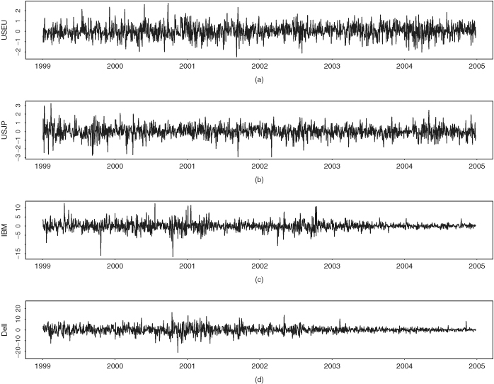
Table 10.1 Descriptive Statistics of Daily Returns of Example 10.6a
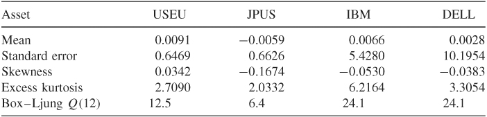
a The returns are in percentages, and the sample period is from January 1999 to December 2004 for 1496 observations.
The equity returns have some serial correlations, but the magnitude is small. If multivariate Ljung–Box statistics are used, we have Q(3) = 59.12 with a p value of 0.13 and Q(5) = 106.44 with a p value of 0.03. For simplicity, we use the sample mean as the mean equation and apply the proposed multivariate volatility model to the mean-corrected data. In estimation, we start with a general model, but add some equality constraints as some estimates appear to be close to each other. The results are given in Table 10.2 along with the value of likelihood function evaluated at the estimates.
Table 10.2 Estimation Results of Multivariate Volatility Models for Example 10.6a

a Lmax denotes the value of likelihood function evaluated at the estimates, v is the degrees of freedom of the multivariate Student-t distribution, and the numbers in parentheses are asymptotic standard errors.
For each estimated multivariate volatility model in Table 10.2, we compute the standardized residuals as
![]()
where ![]() is the symmetric square root matrix of the estimated volatility matrix
is the symmetric square root matrix of the estimated volatility matrix ![]() . We apply the multivariate Ljung–Box statistics to the standardized residuals
. We apply the multivariate Ljung–Box statistics to the standardized residuals ![]() and its squared process
and its squared process ![]() of a fitted model to check model adequacy. For the full model in Table 10.2(a), we have Q(10) = 167.79(0.32) and Q(10) = 110.19(1.00) for
of a fitted model to check model adequacy. For the full model in Table 10.2(a), we have Q(10) = 167.79(0.32) and Q(10) = 110.19(1.00) for ![]() and
and ![]() , respectively, where the number in parentheses denotes p value. Clearly, the model adequately describes the first two moments of the return series. For the model in Table 10.2(b), we have Q(10) = 168.59(0.31) and Q(10) = 109.93(1.00). For the final restricted model in Table 10.2(c), we obtain Q(10) = 168.50(0.31) and Q(10) = 111.75(1.00). Again, the restricted models are capable of describing the mean and volatility of the return series.
, respectively, where the number in parentheses denotes p value. Clearly, the model adequately describes the first two moments of the return series. For the model in Table 10.2(b), we have Q(10) = 168.59(0.31) and Q(10) = 109.93(1.00). For the final restricted model in Table 10.2(c), we obtain Q(10) = 168.50(0.31) and Q(10) = 111.75(1.00). Again, the restricted models are capable of describing the mean and volatility of the return series.
From Table 10.2, we make the following observations. First, using the likelihood ratio test, we cannot reject the final restricted model compared with the full model. This results in a very parsimonious model consisting of only 9 parameters for the time-varying correlations of the four-dimensional return series. Second, for the two stock return series, the constant terms in ![]() are not significantly different from zero, and the sum of GARCH parameters is 0.0372 + 0.9603 = 0.9975, which is very close to unity. Consequently, the volatility series of the two equity returns exhibit IGARCH behavior. On the other hand, the volatility series of the two exchange rate returns appear to have a nonzero constant term and high persistence in GARCH parameters. Third, to better understand the efficacy of the proposed model, we compare the results of the final restricted model with those of rolling estimates. The rolling estimates of covariance matrix are obtained using a moving window of size 69, which is the approximate number of trading days in a quarter. Figure 10.12 shows the time plot of estimated volatility. The solid line is the volatility obtained by the proposed model and the dashed line is for volatility of the rolling estimation. The overall pattern seems similar, but, as expected, the rolling estimates respond more slowly than the proposed model to large innovations. This is shown by the faster rise and decay of the volatility obtained by the proposed model. Figure 10.13 shows the time-varying correlations of the four asset returns. The solid line denotes correlations obtained by the final restricted model of Table 10.2, whereas the dashed line is for rolling estimation. The correlations of the proposed model seem to be smoother.
are not significantly different from zero, and the sum of GARCH parameters is 0.0372 + 0.9603 = 0.9975, which is very close to unity. Consequently, the volatility series of the two equity returns exhibit IGARCH behavior. On the other hand, the volatility series of the two exchange rate returns appear to have a nonzero constant term and high persistence in GARCH parameters. Third, to better understand the efficacy of the proposed model, we compare the results of the final restricted model with those of rolling estimates. The rolling estimates of covariance matrix are obtained using a moving window of size 69, which is the approximate number of trading days in a quarter. Figure 10.12 shows the time plot of estimated volatility. The solid line is the volatility obtained by the proposed model and the dashed line is for volatility of the rolling estimation. The overall pattern seems similar, but, as expected, the rolling estimates respond more slowly than the proposed model to large innovations. This is shown by the faster rise and decay of the volatility obtained by the proposed model. Figure 10.13 shows the time-varying correlations of the four asset returns. The solid line denotes correlations obtained by the final restricted model of Table 10.2, whereas the dashed line is for rolling estimation. The correlations of the proposed model seem to be smoother.
Figure 10.12 Time plots of estimated volatility series of four asset returns. Solid line is from proposed model and dashed line is from a rolling estimation with window size 69: (a) dollar–euro exchange rate, (b) dollar–yen exchange rate, (c) IBM stock, and (d) Dell stock.

Figure 10.13 Time plots of time-varying correlations between percentage simple returns of four assets from January 1999 to December 2004. Solid line is from the proposed model, whereas dashed line is from a rolling estimation with window size 69.

Table 10.2(d) gives the results of a fitted integrated GARCH-type model with leverage effects. The leverage effects are statistically significant for equity returns only and are in the form of an IGARCH model. Specifically, the ![]() matrix of the correlation equation in Eq. (10.31) is
matrix of the correlation equation in Eq. (10.31) is
![]()
Although the magnitudes of the leverage parameters are small, they are statistically significant. This is shown by the likelihood ratio test. Specifically, comparing the fitted models in Table 10.2(b) and (d), the likelihood ratio statistic is 15.16, which has a p value of 0.0005 based on the chi-squared distribution with 2 degrees of freedom.