2.2 Correlation and Autocorrelation Function

The correlation coefficient between two random variables X and Y is defined as

where μx and μy are the mean of X and Y, respectively, and it is assumed that the variances exist. This coefficient measures the strength of linear dependence between X and Y, and it can be shown that − 1 ≤ ρx, y ≤ 1 and ρx, y = ρy, x. The two random variables are uncorrelated if ρx, y = 0. In addition, if both X and Y are normal random variables, then ρx, y = 0 if and only if X and Y are independent. When the sample is available, the correlation can be consistently estimated by its sample counterpart

where and are the sample mean of X and Y, respectively.

Autocorrelation Function (ACF)

Consider a weakly stationary return series rt. When the linear dependence between rt and its past values rt−i is of interest, the concept of correlation is generalized to autocorrelation. The correlation coefficient between rt and rt−ℓ is called the lag-ℓ autocorrelation of rt and is commonly denoted by ρℓ, which under the weak stationarity assumption is a function of ℓ only. Specifically, we define

2.1

where the property Var(rt) = Var(rt−ℓ) for a weakly stationary series is used. From the definition, we have ρ0 = 1, ρℓ = ρ−ℓ, and − 1 ≤ ρℓ ≤ 1. In addition, a weakly stationary series rt is not serially correlated if and only if ρℓ = 0 for all ℓ > 0.

For a given sample of returns , let be the sample mean (i.e., ). Then the lag-1 sample autocorrelation of rt is

Under some general conditions, is a consistent estimate of ρ1. For example, if {rt} is an independent and identically distributed (iid) sequence and , then is asymptotically normal with mean zero and variance 1/T; see Brockwell and Davis (1991, Theorem 7.2.2). This result can be used in practice to test the null hypothesis H0:ρ1 = 0 versus the alternative hypothesis Ha:ρ1 ≠ 0. The test statistic is the usual t ratio, which is and follows asymptotically the standard normal distribution. The null hypothesis H0 is rejected if the t ratio is large in magnitude or, equivalently, the p value of the t ratio is small, say less than 0.05. In general, the lag-ℓ sample autocorrelation of rt is defined as

2.2

If {rt} is an iid sequence satisfying , then is asymptotically normal with mean zero and variance 1/T for any fixed positive integer ℓ. More generally, if rt is a weakly stationary time series satisfying , where ψ0 = 1 and {aj} is a sequence of iid random variables with mean zero, then is asymptotically normal with mean zero and variance for ℓ > q. This is referred to as Bartlett's formula in the time series literature; see Box, Jenkins, and Reinsel (1994). For more information about the asymptotic distribution of sample autocorrelations, see Fuller (1976, Chapter 6) and Brockwell and Davis (1991, Chapter 7).

Testing Individual ACF

For a given positive integer ℓ, the previous result can be used to test H0:ρℓ = 0 vs. Ha:ρℓ ≠ 0. The test statistic is

If {rt} is a stationary Gaussian series satisfying ρj = 0 for j > ℓ, the t ratio is asymptotically distributed as a standard normal random variable. Hence, the decision rule of the test is to reject H0 if |t ratio| > Zα/2, where Zα/2 is the 100(1 − α/2)th percentile of the standard normal distribution. For simplicity, many software packages use 1/T as the asymptotic variance of for all ℓ ≠ 0. They essentially assume that the underlying time series is an iid sequence.

In finite samples, is a biased estimator of ρℓ. The bias is in the order of 1/T, which can be substantial when the sample size T is small. In most financial applications, T is relatively large so that the bias is not serious.

Portmanteau Test

Financial applications often require to test jointly that several autocorrelations of rt are zero. Box and Pierce (1970) propose the Portmanteau statistic

as a test statistic for the null hypothesis H0:ρ1 = ⋯ = ρm = 0 against the alternative hypothesis Ha:ρi ≠ 0 for some i ∈ {1, … , m}. Under the assumption that {rt} is an iid sequence with certain moment conditions, Q*(m) is asymptotically a chi-squared random variable with m degrees of freedom.

Ljung and Box (1978) modify the Q*(m) statistic as below to increase the power of the test in finite samples,

2.3

The decision rule is to reject H0 if , where denotes the 100(1 − α)th percentile of a chi-squared distribution with m degrees of freedom. Most software packages will provide the p value of Q(m). The decision rule is then to reject H0 if the p value is less than or equal to α, the significance level.

In practice, the choice of m may affect the performance of the Q(m) statistic. Several values of m are often used. Simulation studies suggest that the choice of m ≈ ln(T) provides better power performance. This general rule needs modification in analysis of seasonal time series for which autocorrelations with lags at multiples of the seasonality are more important.

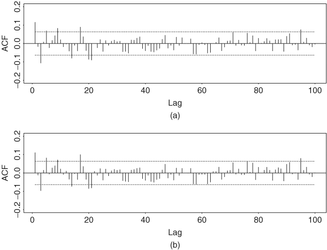
The statistics defined in Eq. (2.2) is called the sample autocorrelation function (ACF) of rt. It plays an important role in linear time series analysis. As a matter of fact, a linear time series model can be characterized by its ACF, and linear time series modeling makes use of the sample ACF to capture the linear dynamic of the data. Figure 2.1 shows the sample autocorrelation functions of monthly simple and log returns of IBM stock from January 1926 to December 2008. The two sample ACFs are very close to each other, and they suggest that the serial correlations of monthly IBM stock returns are very small, if any. The sample ACFs are all within their two standard error limits, indicating that they are not significantly different from zero at the 5% level. In addition, for the simple returns, the Ljung–Box statistics give Q(5) = 3.37 and Q(10) = 13.99, which correspond to p values of 0.64 and 0.17, respectively, based on chi-squared distributions with 5 and 10 degrees of freedom. For the log returns, we have Q(5) = 3.52 and Q(10) = 13.39 with p values 0.62 and 0.20, respectively. The joint tests confirm that monthly IBM stock returns have no significant serial correlations. Figure 2.2 shows the same for the monthly returns of the value-weighted index from the Center for Research in Security Prices (CRSP), at the University of Chicago. There are some significant serial correlations at the 5% level for both return series. The Ljung–Box statistics give Q(5) = 29.71 and Q(10) = 39.55 for the simple returns and Q(5) = 28.38 and Q(10) = 36.16 for the log returns. The p values of these four test statistics are all less than 0.0001, suggesting that monthly returns of the value-weighted index are serially correlated. Thus, the monthly market index return seems to have stronger serial dependence than individual stock returns.

Figure 2.1 Sample autocorrelation functions of monthly (a) simple returns and (b) log returns of IBM stock from January 1926 to December 2008. In each plot, two horizontal dashed lines denote two standard error limits of sample ACF.

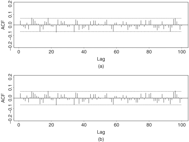
Figure 2.2 Sample autocorrelation functions of monthly (a) simple returns and (b) log returns of value-weighted index of U.S. markets from January 1926 to December 2008. In each plot, two horizontal dashed lines denote two standard error limits of sample ACF.

In the finance literature, a version of the capital asset pricing model (CAPM) theory is that the return {rt} of an asset is not predictable and should have no autocorrelations. Testing for zero autocorrelations has been used as a tool to check the efficient market assumption. However, the way by which stock prices are determined and index returns are calculated might introduce autocorrelations in the observed return series. This is particularly so in analysis of high-frequency financial data. We discuss some of these issues, such as bid–ask bounce and nonsynchronous trading, in Chapter 5.

R Demonstration

The following output has been edited and % denotes explanation:

S-Plus Demonstration

Output edited.