2.4 Simple AR Models

The fact that the monthly return rt of CRSP value-weighted index has a statistically significant lag-1 autocorrelation indicates that the lagged return rt−1 might be useful in predicting rt. A simple model that makes use of such predictive power is

2.8

where {at} is assumed to be a white noise series with mean zero and variance . This model is in the same form as the well-known simple linear regression model in which rt is the dependent variable and rt−1 is the explanatory variable. In the time series literature, model (2.8) is referred to as an autoregressive (AR) model of order 1 or simply an AR(1) model. This simple model is also widely used in stochastic volatility modeling when rt is replaced by its log volatility; see Chapters 3 and 12.

The AR(1) model in Eq. (2.8) has several properties similar to those of the simple linear regression model. However, there are some significant differences between the two models, which we discuss later. Here it suffices to note that an AR(1) model implies that, conditional on the past return rt−1, we have

That is, given the past return rt−1, the current return is centered around ϕ0 + ϕ1rt−1 with standard deviation σa. This is a Markov property such that conditional on rt−1, the return rt is not correlated with rt−i for i > 1. Obviously, there are situations in which rt−1 alone cannot determine the conditional expectation of rt and a more flexible model must be sought. A straightforward generalization of the AR(1) model is the AR(p) model:

2.9

where p is a nonnegative integer and {at} is defined in Eq. (2.8). This model says that the past p variables rt−i (i = 1, … , p) jointly determine the conditional expectation of rt given the past data. The AR(p) model is in the same form as a multiple linear regression model with lagged values serving as the explanatory variables.

2.4.1 Properties of AR Models

For effective use of AR models, it pays to study their basic properties. We discuss properties of AR(1) and AR(2) models in detail and give the results for the general AR(p) model.

AR(1) Model

We begin with the sufficient and necessary condition for weak stationarity of the AR(1) model in Eq. (2.8). Assuming that the series is weakly stationary, we have E(rt) = μ, Var(rt) = γ0, and Cov(rt, rt−j) = γj, where μ and γ0 are constant and γj is a function of j, not t. We can easily obtain the mean, variance, and autocorrelations of the series as follows. Taking the expectation of Eq. (2.8) and because E(at) = 0, we obtain

Under the stationarity condition, E(rt) = E(rt−1) = μ and hence

This result has two implications for rt. First, the mean of rt exists if ϕ1 ≠ 1. Second, the mean of rt is zero if and only if ϕ0 = 0. Thus, for a stationary AR(1) process, the constant term ϕ0 is related to the mean of rt via ϕ0 = (1 − ϕ1)μ and ϕ0 = 0 implies that E(rt) = 0.

Next, using ϕ0 = (1 − ϕ1)μ, the AR(1) model can be rewritten as

2.10

By repeated substitutions, the prior equation implies that

2.11

This equation expresses an AR(1) model in the form of Eq. (2.4) with . Thus, rt − μ is a linear function of at−i for i ≥ 0. Using this property and the independence of the series {at}, we obtain E[(rt − μ)at+1] = 0. By the stationarity assumption, we have Cov(rt−1, at) = E[(rt−1 − μ)at] = 0. This latter result can also be seen from the fact that rt−1 occurred before time t and at does not depend on any past information. Taking the square, then the expectation of Eq. (2.10), we obtain

where is the variance of at, and we make use of the fact that the covariance between rt−1 and at is zero. Under the stationarity assumption, Var(rt) = Var(rt−1), so that

provided that . The requirement of results from the fact that the variance of a random variable is bounded and nonnegative. Consequently, the weak stationarity of an AR(1) model implies that − 1 < ϕ1 < 1, that is, |ϕ1| < 1. Yet if |ϕ1| < 1, then by Eq. (2.11) and the independence of the {at} series, we can show that the mean and variance of rt are finite and time invariant; see Eq. (2.5). In addition, by Eq. (2.6), all the autocovariances of rt are finite. Therefore, the AR(1) model is weakly stationary. In summary, the necessary and sufficient condition for the AR(1) model in Eq. (2.8) to be weakly stationary is |ϕ1| < 1.

Using ϕ0 = (1 − ϕ1)μ, one can rewrite a stationary AR(1) model as

This model is often used in the finance literature with ϕ1 measuring the persistence of the dynamic dependence of an AR(1) time series.

Autocorrelation Function of an AR(1) Model

Multiplying Eq. (2.10) by at, using the independence between at and rt−1, and taking expectation, we obtain

where is the variance of at. Multiplying Eq. (2.10) by rt−ℓ − μ, taking expectation, and using the prior result, we have

where we use γℓ = γ−ℓ. Consequently, for a weakly stationary AR(1) model in Eq. (2.8), we have

From the latter equation, the ACF of rt satisfies

Because ρ0 = 1, we have . This result says that the ACF of a weakly stationary AR(1) series decays exponentially with rate ϕ1 and starting value ρ0 = 1. For a positive ϕ1, the plot of ACF of an AR(1) model shows a nice exponential decay. For a negative ϕ1, the plot consists of two alternating exponential decays with rate . Figure 2.3 shows the ACF of two AR(1) models with ϕ1 = 0.8 and ϕ1 = − 0.8.

AR(2) Model

An AR(2) model assumes the form

2.12

Using the same technique as that of the AR(1) case, we obtain

provided that ϕ1 + ϕ2 ≠ 1. Using ϕ0 = (1 − ϕ1 − ϕ2)μ, we can rewrite the AR(2) model as

Multiplying the prior equation by (rt−ℓ − μ), we have

Taking expectation and using E[(rt−ℓ − μ)at] = 0 for ℓ > 0, we obtain

This result is referred to as the moment equation of a stationary AR(2) model. Dividing the above equation by γ0, we have the property

2.13

for the ACF of rt. In particular, the lag-1 ACF satisfies

Therefore, for a stationary AR(2) series rt, we have ρ0 = 1,

The result of Eq. (2.13) says that the ACF of a stationary AR(2) series satisfies the second-order difference equation

where B is called the back-shift operator such that Bρℓ = ρℓ−1. This difference equation determines the properties of the ACF of a stationary AR(2) time series. It also determines the behavior of the forecasts of rt. In the time series literature, some people use the notation L instead of B for the back-shift operator. Here L stands for lag operator. For instance, Lrt = rt−1 and Lψk = ψk−1.

Corresponding to the prior difference equation, there is a second-order polynomial equation:

2.14

Solutions of this equation are

In the time series literature, inverses of the two solutions are referred to as the characteristic roots of the AR(2) model. Denote the two characteristic roots by ω1 and ω2. If both ωi are real valued, then the second-order difference equation of the model can be factored as (1 − ω1B)(1 − ω2B) and the AR(2) model can be regarded as an AR(1) model operates on top of another AR(1) model. The ACF of rt is then a mixture of two exponential decays. If , then ω1 and ω2 are complex numbers (called a complex-conjugate pair), and the plot of ACF of rt would show a picture of damping sine and cosine waves. In business and economic applications, complex characteristic roots are important. They give rise to the behavior of business cycles. It is then common for economic time series models to have complex-valued characteristic roots. For an AR(2) model in Eq. (2.12) with a pair of complex characteristic roots, the average length of the stochastic cycles is

where the cosine inverse is stated in radians. If one writes the complex solutions as a ± bi, where , then we have ϕ1 = 2a, ϕ2 = − (a2 + b2), and

where is the absolute value of a ± bi. See Example 2.1 for an illustration.

Figure 2.4 shows the ACF of four stationary AR(2) models. Part (b) is the ACF of the AR(2) model (1 − 0.6B + 0.4B2)rt = at. Because , this particular AR(2) model contains two complex characteristic roots, and hence its ACF exhibits damping sine and cosine waves. The other three AR(2) models have real-valued characteristic roots. Their ACFs decay exponentially.

R Demonstration

The R demonstration for Example 2.1, where % denotes explanation, follows:

Stationarity

The stationarity condition of an AR(2) time series is that the absolute values of its two characteristic roots are less than 1, that is, its two characteristic roots are less than 1 in modulus. Equivalently, the two solutions of the characteristic equation are greater than 1 in modulus. Under such a condition, the recursive equation in (2.13) ensures that the ACF of the model converges to 0 as the lag ℓ increases. This convergence property is a necessary condition for a stationary time series. In fact, the condition also applies to the AR(1) model where the polynomial equation is 1 − ϕ1x = 0. The characteristic root is w = 1/x = ϕ1, which must be less than 1 in modulus for rt to be stationary. As shown before, for a stationary AR(1) model. The condition implies that ρℓ → 0 as ℓ → ∞.

AR(p) Model

The results of the AR(1) and AR(2) models can readily be generalized to the general AR(p) model in Eq. (2.9). The mean of a stationary series is

provided that the denominator is not zero. The associated characteristic equation of the model is

If all the solutions of this equation are greater than 1 in modulus, then the series rt is stationary. Again, inverses of the solutions are the characteristic roots of the model. Thus, stationarity requires that all characteristic roots are less than 1 in modulus. For a stationary AR(p) series, the ACF satisfies the difference equation

The plot of ACF of a stationary AR(p) model would then show a mixture of damping sine and cosine patterns and exponential decays depending on the nature of its characteristic roots.

2.4.2 Identifying AR Models in Practice

In application, the order p of an AR time series is unknown. It must be specified empirically. This is referred to as the order determination (or order specification) of AR models, and it has been extensively studied in the time series literature. Two general approaches are available for determining the value of p. The first approach is to use the partial autocorrelation function, and the second approach uses some information criteria.

Partial Autocorrelation Function (PACF)

The PACF of a stationary time series is a function of its ACF and is a useful tool for determining the order p of an AR model. A simple, yet effective way to introduce PACF is to consider the following AR models in consecutive orders:

where ϕ0, j, ϕi, j, and {ejt} are, respectively, the constant term, the coefficient of rt−i, and the error term of an AR(j) model. These models are in the form of a multiple linear regression and can be estimated by the least-squares method. As a matter of fact, they are arranged in a sequential order that enables us to apply the idea of partial F test in multiple linear regression analysis. The estimate of the first equation is called the lag-1 sample PACF of rt. The estimate of the second equation is the lag-2 sample PACF of rt. The estimate of the third equation is the lag-3 sample PACF of rt, and so on.

From the definition, the lag-2 PACF shows the added contribution of rt−2 to rt over the AR(1) model rt = ϕ0 + ϕ1rt−1 + e1t. The lag-3 PACF shows the added contribution of rt−3 to rt over an AR(2) model, and so on. Therefore, for an AR(p) model, the lag-p sample PACF should not be zero, but should be close to zero for all j > p. We make use of this property to determine the order p. For a stationary Gaussian AR(p) model, it can be shown that the sample PACF has the following properties:

• converges to ϕp as the sample size T goes to infinity.
• converges to zero for all ℓ > p.
• The asymptotic variance of is 1/T for ℓ > p.

These results say that, for an AR(p) series, the sample PACF cuts off at lag p.

As an example, consider the monthly simple returns of CRSP value-weighted index from January 1926 to December 2008. Table 2.1 gives the first 12 lags of sample PACF of the series. With T = 996, the asymptotic standard error of the sample PACF is approximately 0.032. Therefore, using the 5% significant level, we identify an AR(3) or AR(9) model for the data (i.e., p = 3 or 9). If the 1% significant level is used, we specify an AR(3) model.

Table 2.1 Sample Partial Autocorrelation Function and Some Information Criteria for the Monthly Simple Returns of CRSP Value-Weighted Index from January 1926 to December 2008

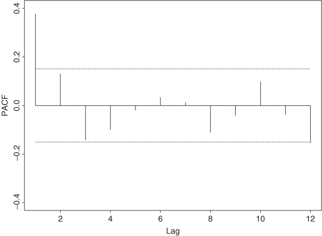
As another example, Figure 2.6 shows the PACF of the GNP growth rate series of Example 2.1. The two dotted lines of the plot denote the approximate two standard error limits . The plot suggests an AR(3) model for the data because the first three lags of sample PACF appear to be large.

Information Criteria

There are several information criteria available to determine the order p of an AR process. All of them are likelihood based. For example, the well-known Akaike information criterion (AIC) (Akaike, 1973) is defined as

2.16

where the likelihood function is evaluated at the maximum-likelihood estimates and T is the sample size. For a Gaussian AR(ℓ) model, AIC reduces to

where is the maximum-likelihood estimate of , which is the variance of at, and T is the sample size; see Eq. (1.18). The first term of the AIC in Eq. (2.16) measures the goodness of fit of the AR(ℓ) model to the data, whereas the second term is called the penalty function of the criterion because it penalizes a candidate model by the number of parameters used. Different penalty functions result in different information criteria.

Another commonly used criterion function is the Schwarz–Bayesian information criterion (BIC). For a Gaussian AR(ℓ) model, the criterion is

The penalty for each parameter used is 2 for AIC and ln(T) for BIC. Thus, compared with AIC, BIC tends to select a lower AR model when the sample size is moderate or large.

Selection Rule

To use AIC to select an AR model in practice, one computes AIC(ℓ) for ℓ = 0, … , P, where p is a prespecified positive integer and selects the order k that has the minimum AIC value. The same rule applies to BIC.

Table 2.1 also gives the AIC and BIC for p = 1, … , 12. The AIC values are close to each other with minimum − 5.849 occurring at p = 9, suggesting that an AR(9) model is preferred by the criterion. The BIC, on the other hand, attains its minimum value − 5.833 at p = 1 with − 5.831 as a close second at p = 3. Thus, the BIC selects an AR(1) model for the value-weighted return series. This example shows that different approaches or criteria to order determination may result in different choices of p. There is no evidence to suggest that one approach outperforms the other in a real application. Substantive information of the problem under study and simplicity are two factors that also play an important role in choosing an AR model for a given time series.

Again, consider the growth rate series of U.S. quarterly real GNP of Example 2.1. The AIC obtained from R also identifies an AR(3) model. Note that the AIC value of the ar command in R has been adjusted so that the minimum AIC is zero.

Parameter Estimation

For a specified AR(p) model in Eq. (2.9), the conditional least-squares method, which starts with the (p + 1)th observation, is often used to estimate the parameters. Specifically, conditioning on the first p observations, we have

which is in the form of a multiple linear regression and can be estimated by the least-squares method. Denote the estimate of ϕi by . The fitted model is

and the associated residual is

The series {ât} is called the residual series, from which we obtain

If the conditional-likelihood method is used, the estimates of ϕi remain unchanged, but the estimate of becomes . In some packages, is defined as . For illustration, consider an AR(3) model for the monthly simple returns of the value-weighted index in Table 2.1. The fitted model is

The standard errors of the coefficients are 0.002, 0.032, 0.032, and 0.032, respectively. Except for the lag-2 coefficient, all parameters are statistically significant at the 1% level.

For this example, the AR coefficients of the fitted model are small, indicating that the serial dependence of the series is weak, even though it is statistically significant at the 1% level. The significance of of the entertained model implies that the expected mean return of the series is positive. In fact, , which is small but has an important long-term implication. It implies that the long-term return of the index can be substantial. Using the multiperiod simple return defined in Chapter 1, the average annual simple gross return is . In other words, the monthly simple returns of the CRSP value-weighted index grew about 9.3% per annum from 1926 to 2008, supporting the common belief that equity market performs well in the long term. A one-dollar investment at the beginning of 1926 would be worth about $1593 at the end of 2008.

Model Checking

A fitted model must be examined carefully to check for possible model inadequacy. If the model is adequate, then the residual series should behave as a white noise. The ACF and the Ljung–Box statistics in Eq. (2.3) of the residuals can be used to check the closeness of ât to a white noise. For an AR(p) model, the Ljung–Box statistic Q(m) follows asymptotically a chi-squared distribution with m − g degrees of freedom, where g denotes the number of AR coefficients used in the model. The adjustment in the degrees of freedom is made based on the number of constraints added to the residuals ât from fitting the AR(p) to an AR(0) model. If a fitted model is found to be inadequate, it must be refined. For instance, if some of the estimated AR coefficients are not significantly different from zero, then the model should be simplified by trying to remove those insignificant parameters. If residual ACF shows additional serial correlations, then the model should be extended to take care of those correlations.

Consider the residual series of the fitted AR(3) model for the monthly value-weighted simple returns. We have Q(12) = 16.35 with a p value 0.060 based on its asymptotic chi-squared distribution with 9 degrees of freedom. Thus, the null hypothesis of no residual serial correlation in the first 12 lags is barely not rejected at the 5% level. However, since the lag-2 AR coefficient is not significant at the 5% level, one can refine the model as

where all the estimates are now significant at the 1% level. The residual series gives Q(12) = 16.83 with a p value 0.078 (based on ). The model is adequate in modeling the dynamic linear dependence of the data.

R Demonstration

In the following R demonstration, % denotes an explanation:

S-Plus Demonstration

The following S-Plus output has been edited:

2.4.3 Goodness of Fit

A commonly used statistic to measure goodness of fit of a stationary model is the R square (R2) defined as

For a stationary AR(p) time series model with T observations {rt|t = 1, … , T}, the measure becomes

where . It is easy to show that 0 ≤ R2 ≤ 1. Typically, a larger R2 indicates that the model provides a closer fit to the data. However, this is only true for a stationary time series. For the unit-root nonstationary series discussed later in this chapter, R2 of an AR(1) fit converges to one when the sample size increases to infinity, regardless of the true underlying model of rt.

For a given data set, it is well known that R2 is a nondecreasing function of the number of parameters used. To overcome this weakness, an adjusted R2 is proposed, which is defined as

where is the sample variance of rt. This new measure takes into account the number of parameters used in the fitted model. However, it is no longer between 0 and 1.

2.4.4 Forecasting

Forecasting is an important application of time series analysis. For the AR(p) model in Eq. (2.9), suppose that we are at the time index h and are interested in forecasting rh+ℓ, where ℓ ≥ 1. The time index h is called the forecast origin and the positive integer ℓ is the forecast horizon. Let be the forecast of rh+ℓ using the minimum squared error loss function. In other words, the forecast is chosen such that

where g is a function of the information available at time h (inclusive), that is, a function of Fh. We referred to as the ℓ-step ahead forecast of rt at the forecast origin h. Let Fh be the collection of information available at the forecast origin h.

1-Step-Ahead Forecast

From the AR(p) model, we have

Under the minimum squared error loss function, the point forecast of rh+1 given Fh is the conditional expectation

and the associated forecast error is

Consequently, the variance of the 1-step-ahead forecast error is Var[eh(1)] = Var(ah+1) = . If at is normally distributed, then a 95% 1-step-ahead interval forecast of rh+1 is . For the linear model in Eq. (2.4), at+1 is also the 1-step-ahead forecast error at the forecast origin t. In the econometric literature, at+1 is referred to as the shock to the series at time t + 1.

In practice, estimated parameters are often used to compute point and interval forecasts. This results in a conditional forecast because such a forecast does not take into consideration the uncertainty in the parameter estimates. In theory, one can consider parameter uncertainty in forecasting, but it is much more involved. A natural way to consider parameter and model uncertainty in forecasting is Bayesian forecasting with Markov chan Monte Carlo (MCMC) methods. See Chapter 12 for further discussion. For simplicity, we assume that the model is given in this chapter. When the sample size used in estimation is sufficiently large, then the conditional forecast is close to the unconditional one.

2-Step-Ahead Forecast

Next consider the forecast of rh+2 at the forecast origin h. From the AR(p) model, we have

Taking conditional expectation, we have

and the associated forecast error

The variance of the forecast error is Var[eh(2)] = . Interval forecasts of rh+2 can be computed in the same way as those for rh+1. It is interesting to see that Var[eh(2)] ≥ Var[eh(1)], meaning that as the forecast horizon increases the uncertainty in forecast also increases. This is in agreement with common sense that we are more uncertain about rh+2 than rh+1 at the time index h for a linear time series.

Multistep-Ahead Forecast

In general, we have

The ℓ-step-ahead forecast based on the minimum squared error loss function is the conditional expectation of rh+ℓ given Fh, which can be obtained as

where it is understood that if i ≤ 0. This forecast can be computed recursively using forecasts for i = 1, … , ℓ − 1. The ℓ-step-ahead forecast error is . It can be shown that for a stationary AR(p) model, converges to E(rt) as ℓ → ∞, meaning that for such a series long-term point forecast approaches its unconditional mean. This property is referred to as the mean reversion in the finance literature. For an AR(1) model, the speed of mean reversion is measured by the half-life defined as ℓ = ln(0.5)/ln(|ϕ1|). The variance of the forecast error then approaches the unconditional variance of rt. Note that for an AR(1) model in (2.8), let xt = rt − E(rt) be the mean-adjusted series. It is easy to see that the ℓ-step-ahead forecast of xh+ℓ at the forecast orign h is . The half-life is the forecast horizon such that . That is, . Thus, ℓ = ln(0.5)/ln(|ϕ1|).

Table 2.2 contains the 1-step- to 12-step ahead forecasts and the standard errors of the associated forecast errors at the forecast origin 984 for the monthly simple return of the value-weighted index using an AR(3) model that was reestimated using the first 984 observations. The fitted model is

where . The actual returns of 2008 are also given in Table 2.2. Because of the weak serial dependence in the series, the forecasts and standard deviations of forecast errors converge to the sample mean and standard deviation of the data quickly. For the first 984 observations, the sample mean and standard error are 0.0095 and 0.0540, respectively.

Table 2.2 Multistep Ahead Forecasts of an AR(3) Model for Monthly Simple Returns of CRSP Value-Weighted Index

aThe forecast origin is h = 984.

Figure 2.7 shows the corresponding out-of-sample prediction plot for the monthly simple return series of the value-weighted index. The forecast origin t = 984 corresponds to December 2007. The prediction plot includes the two standard error limits of the forecasts and the actual observed returns for 2008. The forecasts and actual returns are marked by ° and •, respectively. From the plot, except for the return of October 2008, all actual returns are within the 95% prediction intervals.