2.3 White Noise and Linear Time Series

White Noise

A time series rt is called a white noise if {rt} is a sequence of independent and identically distributed random variables with finite mean and variance. In particular, if rt is normally distributed with mean zero and variance σ2, the series is called a Gaussian white noise. For a white noise series, all the ACFs are zero. In practice, if all sample ACFs are close to zero, then the series is a white noise series. Based on Figures 2.1 and 2.2, the monthly returns of IBM stock are close to white noise, whereas those of the value-weighted index are not.

The behavior of sample autocorrelations of the value-weighted index returns indicates that for some asset returns it is necessary to model the serial dependence before further analysis can be made. In what follows, we discuss some simple time series models that are useful in modeling the dynamic structure of a time series. The concepts presented are also useful later in modeling volatility of asset returns.

Linear Time Series

A time series rt is said to be linear if it can be written as

2.4

where μ is the mean of rt, ψ0 = 1, and {at} is a sequence of iid random variables with mean zero and a well-defined distribution (i.e., {at} is a white noise series). It will be seen later that at denotes the new information at time t of the time series and is often referred to as the innovation or shock at time t. In this book, we are mainly concerned with the case where at is a continuous random variable. Not all financial time series are linear, however. We study nonlinearity and nonlinear models in Chapter 4.

For a linear time series in Eq. (2.4), the dynamic structure of rt is governed by the coefficients ψi, which are called the ψ weights of rt in the time series literature. If rt is weakly stationary, we can obtain its mean and variance easily by using the independence of {at} as

2.5

where is the variance of at. Because Var(rt) < ∞, must be a convergent sequence, that is, as i → ∞. Consequently, for a stationary series, impact of the remote shock at−i on the return rt vanishes as i increases.

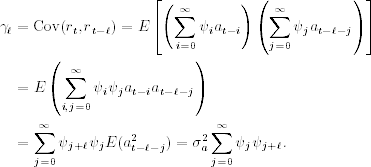
The lag-ℓ autocovariance of rt is

2.6

Consequently, the ψ weights are related to the autocorrelations of rt as follows:

2.7

where ψ0 = 1. Linear time series models are econometric and statistical models used to describe the pattern of the ψ weights of rt. For a weakly stationary time series, ψi → 0 as i → ∞ and, hence, ρℓ converges to zero as ℓ increases. For asset returns, this means that, as expected, the linear dependence of current return rt on the remote past return rt−ℓ diminishes for large ℓ.