
9.5 Statistical Factor Analysis
We now turn to statistical factor analysis. One of the main difficulties in multivariate statistical analysis is the “curse of dimensionality.” For serially correlated data, the number of parameters of a parametric model often increases dramatically when the order of the model or the dimension of the time series is increased. Simplifying methods are often sought to overcome the curse of dimensionality. From an empirical viewpoint, multivariate data often exhibit similar patterns indicating the existence of common structure hidden in the data. Statistical factor analysis is one of those simplifying methods available in the literature. The aim of statistical factor analysis is to identify, from the observed data, a few factors that can account for most of the variations in the covariance or correlation matrix of the data.
Traditional statistical factor analysis assumes that the data have no serial correlations. This assumption is often violated by financial data taken with frequency less than or equal to a week. However, the assumption appears to be reasonable for asset returns with lower frequencies (e.g., monthly returns of stocks or market indexes). If the assumption is violated, then one can use the parametric models discussed in this book to remove the linear dynamic dependence of the data and apply factor analysis to the residual series.
In what follows, we discuss statistical factor analysis based on the orthogonal factor model. Consider the return ![]() of k assets at time period t and assume that the return series
of k assets at time period t and assume that the return series ![]() is weakly stationary with mean
is weakly stationary with mean ![]() and covariance matrix
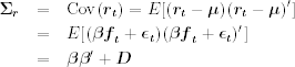
and covariance matrix ![]() . The statistical factor model postulates that
. The statistical factor model postulates that ![]() is linearly dependent on a few unobservable random variables
is linearly dependent on a few unobservable random variables ![]() and k additional noises
and k additional noises ![]() = (ϵ1t, … , ϵkt)′. Here m < k, fit are the common factors, and ϵit are the errors. Mathematically, the statistical factor model is also in the form of Eq. (9.1) except that the intercept
= (ϵ1t, … , ϵkt)′. Here m < k, fit are the common factors, and ϵit are the errors. Mathematically, the statistical factor model is also in the form of Eq. (9.1) except that the intercept ![]() is replaced by the mean return
is replaced by the mean return ![]() . Thus, a statistical factor model is in the form
. Thus, a statistical factor model is in the form
where ![]() is the matrix of factor loadings, βij is the loading of the ith variable on the jth factor, and ϵit is the specific error of rit. A key feature of the statistical factor model is that the m factors fit and the factor loadings βij are unobservable. As such, Eq. (9.16) is not a multivariate linear regression model, even though it has a similar appearance. This special feature also distinguishes a statistical factor model from other factor models discussed earlier.
is the matrix of factor loadings, βij is the loading of the ith variable on the jth factor, and ϵit is the specific error of rit. A key feature of the statistical factor model is that the m factors fit and the factor loadings βij are unobservable. As such, Eq. (9.16) is not a multivariate linear regression model, even though it has a similar appearance. This special feature also distinguishes a statistical factor model from other factor models discussed earlier.
The factor model in Eq. (9.16) is an orthogonal factor model if it satisfies the following assumptions:
1. ![]() and Cov(
and Cov(![]() ) =
) = ![]() , the m × m identity matrix.
, the m × m identity matrix.
2. ![]() and
and ![]() = diag
= diag![]() (i.e.,
(i.e., ![]() is a k × k diagonal matrix).
is a k × k diagonal matrix).
3. ![]() and
and ![]() are independent so that Cov(
are independent so that Cov(![]() ) =
) = ![]() .
.
Under the previous assumptions, it is easy to see that
and
Using Eqs. (9.17) and (9.18), we see that for the orthogonal factor model in Eq. (9.16)

The quantity ![]() , which is the portion of the variance of rit contributed by the m common factors, is called the communality. The remaining portion
, which is the portion of the variance of rit contributed by the m common factors, is called the communality. The remaining portion ![]() of the variance of rit is called the uniqueness or specific variance. Let
of the variance of rit is called the uniqueness or specific variance. Let ![]() be the communality, which is the sum of squares of the loadings of the ith variable on the m common factors. The variance of component rit becomes
be the communality, which is the sum of squares of the loadings of the ith variable on the m common factors. The variance of component rit becomes ![]() .
.
In practice, not every covariance matrix has an orthogonal factor representation. In other words, there exists a random variable ![]() that does not have any orthogonal factor representation. Furthermore, the orthogonal factor representation of a random variable is not unique. In fact, for any m × m orthogonal matrix
that does not have any orthogonal factor representation. Furthermore, the orthogonal factor representation of a random variable is not unique. In fact, for any m × m orthogonal matrix ![]() satisfying
satisfying ![]() =
= ![]() =
= ![]() , let
, let ![]() and
and ![]() . Then
. Then
![]()
In addition, ![]() and
and ![]()
![]() . Thus,
. Thus, ![]() and
and ![]() form another orthogonal factor model for
form another orthogonal factor model for ![]() . This nonuniqueness of orthogonal factor representation is a weakness as well as an advantage for factor analysis. It is a weakness because it makes the meaning of factor loading arbitrary. It is an advantage because it allows us to perform rotations to find common factors that have nice interpretations. Because
. This nonuniqueness of orthogonal factor representation is a weakness as well as an advantage for factor analysis. It is a weakness because it makes the meaning of factor loading arbitrary. It is an advantage because it allows us to perform rotations to find common factors that have nice interpretations. Because ![]() is an orthogonal matrix, the transformation
is an orthogonal matrix, the transformation ![]() is a rotation in the m-dimensional space.
is a rotation in the m-dimensional space.
9.5.1 Estimation
The orthogonal factor model in Eq. (9.16) can be estimated by two methods. The first estimation method uses the principal component analysis of the previous section. This method does not require the normality assumption of the data nor the prespecification of the number of common factors. It applies to both the covariance and correlation matrices. But as mentioned in PCA, the solution is often an approximation. The second estimation method is the maximum-likelihood method that uses normal density and requires a prespecification for the number of common factors.
9.5.1.1 Principal Component Method
Again let ![]() be pairs of the eigenvalues and eigenvectors of the sample covariance matrix
be pairs of the eigenvalues and eigenvectors of the sample covariance matrix ![]() , where
, where ![]() . Let m < k be the number of common factors. Then the matrix of factor loadings is given by
. Let m < k be the number of common factors. Then the matrix of factor loadings is given by
The estimated specific variances are the diagonal elements of the matrix ![]() . That is,
. That is, ![]() = diag
= diag![]() , where
, where ![]() , where
, where ![]() is the (i, i)th element of
is the (i, i)th element of ![]() . The communalities are estimated by
. The communalities are estimated by
![]()
The error matrix caused by approximation is
![]()
Ideally, we would like this matrix to be close to zero. It can be shown that the sum of squared elements of ![]() is less than or equal to
is less than or equal to ![]() . Therefore, the approximation error is bounded by the sum of squares of the neglected eigenvalues.
. Therefore, the approximation error is bounded by the sum of squares of the neglected eigenvalues.
From the solution in Eq. (9.19), the estimated factor loadings based on the principal component method do not change as the number of common factors m is increased.
9.5.1.2 Maximum-Likelihood Method
If the common factors ![]() and the specific factors
and the specific factors ![]() are jointly normal, then
are jointly normal, then ![]() is multivariate normal with mean
is multivariate normal with mean ![]() and covariance matrix
and covariance matrix ![]() =
= ![]() . The maximum-likelihood method can then be used to obtain estimates of
. The maximum-likelihood method can then be used to obtain estimates of ![]() and
and ![]() under the constraint
under the constraint ![]() =
= ![]() , which is a diagonal matrix. Here
, which is a diagonal matrix. Here ![]() is estimated by the sample mean. For more details of this method, readers are referred to Johnson and Wichern (2007).
is estimated by the sample mean. For more details of this method, readers are referred to Johnson and Wichern (2007).
In using the maximum-likelihood method, the number of common factors must be given a priori. In practice, one can use a modified likelihood ratio test to check the adequacy of a fitted m-factor model. The test statistic is
which, under the null hypothesis of m factors, is asymptotically distributed as a chi-squared distribution with ![]() degrees of freedom. We discuss some methods for selecting m in Section 9.6.1.
degrees of freedom. We discuss some methods for selecting m in Section 9.6.1.
9.5.2 Factor Rotation
As mentioned before, for any m × m orthogonal matrix ![]() ,
,
![]()
where ![]() and
and ![]() . In addition,
. In addition,
![]()
This result indicates that the communalities and the specific variances remain unchanged under an orthogonal transformation. It is then reasonable to find an orthogonal matrix ![]() to transform the factor model so that the common factors have nice interpretations. Such a transformation is equivalent to rotating the common factors in the m-dimensional space. In fact, there are infinite possible factor rotations available. Kaiser (1958) proposes a varimax criterion to select the rotation that works well in many applications. Denote the rotated matrix of factor loadings by
to transform the factor model so that the common factors have nice interpretations. Such a transformation is equivalent to rotating the common factors in the m-dimensional space. In fact, there are infinite possible factor rotations available. Kaiser (1958) proposes a varimax criterion to select the rotation that works well in many applications. Denote the rotated matrix of factor loadings by ![]() =
= ![]() and the ith communality by
and the ith communality by ![]() . Define
. Define ![]() to be the rotated coefficients scaled by the (positive) square root of communalities. The varimax procedure selects the orthogonal matrix
to be the rotated coefficients scaled by the (positive) square root of communalities. The varimax procedure selects the orthogonal matrix ![]() that maximizes the quantity
that maximizes the quantity
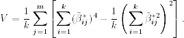
This complicated expression has a simple interpretation. Maximizing V corresponds to spreading out the squares of the loadings on each factor as much as possible. Consequently, the procedure is to find groups of large and negligible coefficients in any column of the rotated matrix of factor loadings. In a real application, factor rotation is used to aid the interpretations of common factors. It may be helpful in some applications, but not informative in others. There are many criteria available for factor rotation.
9.5.3 Applications
Given the data ![]() of asset returns, the statistical factor analysis enables us to search for common factors that explain the variabilities of the returns. Since factor analysis assumes no serial correlations in the data, one should check the validity of this assumption before using factor analysis. The multivariate portmanteau statistics can be used for this purpose. If serial correlations are found, one can build a VARMA model to remove the dynamic dependence in the data and apply the factor analysis to the residual series. For many returns series, the correlation matrix of the residuals of a linear model is often very close to the correlation matrix of the original data. In this case, the effect of dynamic dependence on factor analysis is negligible.
of asset returns, the statistical factor analysis enables us to search for common factors that explain the variabilities of the returns. Since factor analysis assumes no serial correlations in the data, one should check the validity of this assumption before using factor analysis. The multivariate portmanteau statistics can be used for this purpose. If serial correlations are found, one can build a VARMA model to remove the dynamic dependence in the data and apply the factor analysis to the residual series. For many returns series, the correlation matrix of the residuals of a linear model is often very close to the correlation matrix of the original data. In this case, the effect of dynamic dependence on factor analysis is negligible.
We consider three examples in this section. The first and third examples use the R or S-Plus to perform the analysis and the second example uses Minitab. Other packages can also be used.
Example 9.2
Consider again the monthly log stock returns of IBM, Hewlett-Parkard, Intel, J.P. Morgan Chase, and Bank of America used in Example 9.1. To check the assumption of no serial correlations, we compute the portmanteau statistics and obtain Q5(1) = 39.99, Q5(5) = 160.60, and Q5(10) = 293.04. Compared with chi-squared distributions with 25, 125, and 250 degrees of freedom, the p values of these test statistics are 0.029, 0.017, and 0.032, respectively. Therefore, there exists some minor serial dependence in the returns, but the dependence is not significant at the 1% level. For simplicity, we ignore the serial dependence in factor analysis.
Table 9.4 shows the results of factor analysis based on the correlation matrix using the maximum-likelihood method. We assume that the number of common factors is 2, which is reasonable according to the principal component analysis of Example 9.1. From the table, the factor analysis reveals several interesting findings:
- The two factors identified by the maximum-likelihood method explain about 60% of the variability of the stock returns.
- Based on the rotated factor loadings, the two common factors have some meaningful interpretations. The technology stocks (IBM, Hewlett-Packard, and Intel) load heavily on the first factor, whereas the financial stocks (J.P. Morgan Chase and Bank of America) load highly on the second factor. These two rotated factors jointly differentiate the industrial sectors.
- In this particular instance, the varimax rotation seems to alter the ordering of the two common factors.
- The specific variance of IBM stock returns is relatively large, indicating that the stock has its own features that are worth further investigation.
Example 9.3
In this example, we consider the monthly log returns of U.S. bond indexes with maturities in 30 years, 20 years, 10 years, 5 years, and 1 year. The data are described in Example 8.2 but have been transformed into log returns. There are 696 observations. As shown in Example 8.2, there is serial dependence in the data. However, removing serial dependence by fitting a VARMA(2,1) model has hardly any effects on the concurrent correlation matrix. As a matter of fact, the correlation matrices before and after fitting a VARMA(2,1) model are
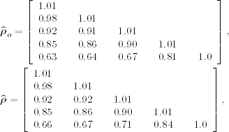
where ![]() is the correlation matrix of the original log returns. Therefore, we apply factor analysis directly to the return series.
is the correlation matrix of the original log returns. Therefore, we apply factor analysis directly to the return series.
Table 9.4 Factor Analysis of Monthly Log Stock Returns of IBM, Hewlett-Packard, Intel, J.P. Morgan Chase, and Bank of Americaa
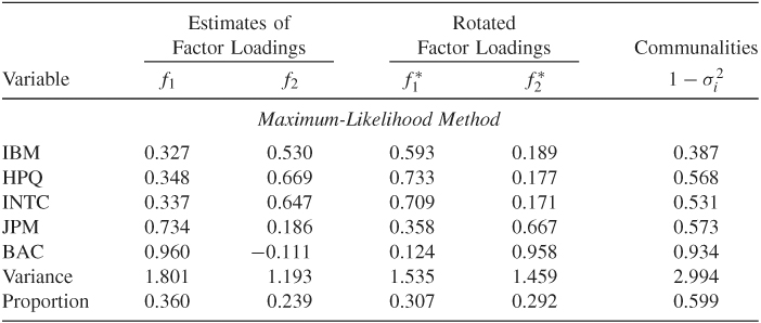
aThe returns include dividends and are from January 1990 to December 2008. The analysis is based on the sample cross-correlation matrix and assumes two common factors.
Table 9.5 shows the results of statistical factor analysis of the data. For both estimation methods, the first two common factors explain more than 90% of the total variability of the data. Indeed, the high communalities indicate that the specific variances are very small for the five bond index returns. Because the results of the two methods are close, we only discuss that of the principal component method. The unrotated factor loadings indicate that (a) all five return series load roughly equally on the first factor, and (b) the loadings on the second factor are positively correlated with the time to maturity. Therefore, the first common factor represents the general U.S. bond returns, and the second factor shows the “time-to-maturity” effect. Furthermore, the loadings of the second factor sum approximately to zero. Therefore, this common factor can also be interpreted as the contrast between long-term and short-term bonds. Here a long-term bond means one with maturity 10 years or longer. For the rotated factors, the loadings are also interesting. The loadings for the first rotated factor are proportional to the time to maturity, whereas the loadings of the second factor are inversely proportional to the time to maturity.
Table 9.5 Factor Analysis of Monthly Log Returns of U.S. Bond Indexes with Maturities in 30 Years, 20 Years, 10 Years, 5 Years, and 1 Yeara
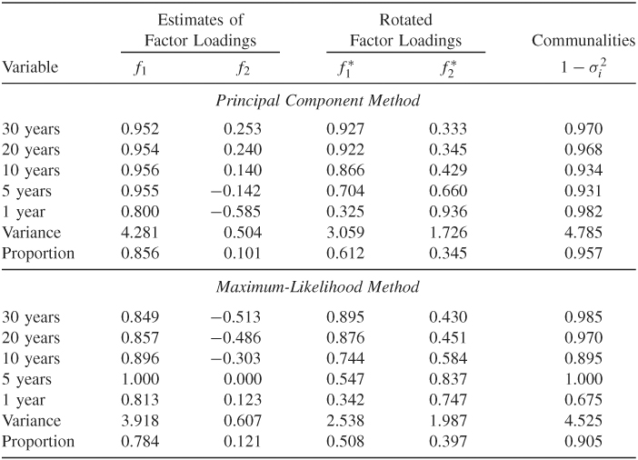
aThe data are from January 1942 to December 1999. The analysis is based on the sample cross-correlation matrix and assumes two common factors.
Example 9.4
Again, consider the monthly excess returns of the 10 stocks in Table 9.2. The sample span is from January 1990 to December 2003 and the returns are in percentages. Our goal here is to demonstrate the use of statistical factor models using the R or S-Plus command factanal. We started with a two-factor model, but it is rejected by the likelihood ratio test of Eq. (9.20). The test statistic is LR(2) = 72.96. Based on the asymptotic ![]() distribution, p value of the test statistic is close to zero.
distribution, p value of the test statistic is close to zero.
> rtn=read.table(“m-barra-9003.txt”,header=T)
> stat.fac=factanal(rtn,factors=2,method=‘mle’)
> stat.fac
Sums of squares of loadings:
Factor1 Factor2
2.696479 2.19149
Component names:
“loadings” “uniquenesses” “correlation” “criteria”
“factors” “dof” “method” “center” “scale” “n.obs”
“scores” “call”
We then applied a three-factor model that appears to be reasonable at the 5% significance level. The p value of the LR(3) statistic is 0.0892.
> stat.fac=factanal(rtn,factor=3,method=‘mle’)
> stat.fac
Test of the hypothesis that 3 factors are sufficient
versus the alternative that more are required:
The chi square statistic is 26.48 on 18 degrees of freedom.
The p-value is 0.0892
> summary(stat.fac)
Importance of factors:
Factor1 Factor2 Factor3
SS loadings 2.635 1.825 1.326
Proportion Var 0.264 0.183 0.133
Cumulative Var 0.264 0.446 0.579
Uniquenesses:
AGE C MWD MER DELL HPQ IBM
0.479 0.341 0.201 0.216 0.690 0.346 0.638
AA CAT PG
0.417 0.000 0.885
Loadings:
Factor1 Factor2 Factor3
AGE 0.678 0.217 0.121
C 0.739 0.259 0.213
MWD 0.817 0.356
MER 0.819 0.329
DELL 0.102 0.547
HPQ 0.230 0.771
IBM 0.200 0.515 0.238
AA 0.194 0.546 0.497
CAT 0.198 0.138 0.970
PG 0.331
The factor loadings can also be shown graphically using
> plot(loadings(stat.fac))
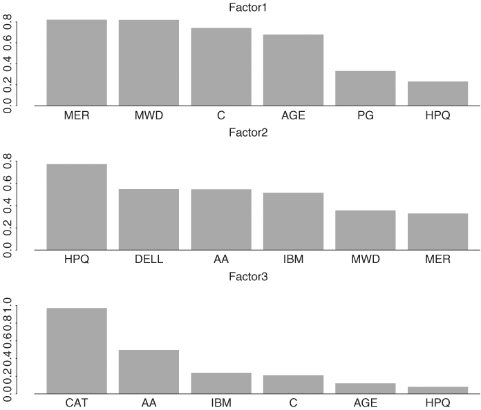
and the plots are in Figure 9.6. From the plots, factor 1 represents essentially the financial service sector, and factor 2 mainly consists of the excess returns from the high-tech stocks and the Alcoa stock. Factor 3 depends heavily on excess returns of CAT and AA stocks and, hence, represents the remaining industrial sector.
Figure 9.6 Plots of factor loadings when a 3-factor statistical factor model is fitted to 10 monthly excess stock returns in Table 9.2.
Factor rotation can be obtained using the command rotate, which allows for many rotation methods, and factor realizations are available from the command predict.
> stat.fac2 = rotate(stat.fac,rotation=‘quartimax’)
> loadings(stat.fac2)
Factor1 Factor2 Factor3
AGE 0.700 0.171
C 0.772 0.216 0.124
MWD 0.844 0.291
MER 0.844 0.264
DELL 0.144 0.536
HPQ 0.294 0.753
IBM 0.258 0.518 0.164
AA 0.278 0.575 0.418
CAT 0.293 0.219 0.931
PG 0.334
> factor.real=predict(stat.fac,type=‘weighted.ls’)
Finally, we obtained the correlation matrix of the 10 excess returns based on the fitted three-factor statistical factor model. As expected, the correlations are closer to their sample counterparts than those of the industrial factor model in Section 9.3.1. One can also use GMVP to compare the covariance matrices of the returns and the statistical factor model.
> corr.fit=fitted(stat.fac)
> print(corr.fit,digits=1,width=2)
AGE C MWD MER DELL HPQ IBM AA CAT PG
AGE 1.0 0.6 0.6 0.6 0.19 0.3 0.3 0.3 0.3 0.2
C 0.6 1.0 0.7 0.7 0.22 0.4 0.3 0.4 0.4 0.3
MWD 0.6 0.7 1.0 0.8 0.28 0.5 0.4 0.4 0.3 0.3
MER 0.6 0.7 0.8 1.0 0.26 0.5 0.4 0.4 0.3 0.3
DELL 0.2 0.2 0.3 0.3 1.00 0.5 0.3 0.3 0.1 0.0
HPQ 0.3 0.4 0.5 0.4 0.45 1.0 0.5 0.5 0.2 0.1
IBM 0.3 0.3 0.4 0.3 0.31 0.5 1.0 0.4 0.3 0.1
AA 0.3 0.4 0.4 0.4 0.33 0.5 0.4 1.0 0.6 0.1
CAT 0.3 0.4 0.3 0.3 0.11 0.2 0.3 0.6 1.0 0.1
PG 0.2 0.3 0.3 0.3 0.03 0.1 0.1 0.1 0.1 1.0