2.6 Simple ARMA Models

In some applications, the AR or MA models discussed in the previous sections become cumbersome because one may need a high-order model with many parameters to adequately describe the dynamic structure of the data. To overcome this difficulty, the autoregressive moving-average (ARMA) models are introduced; see Box, Jenkins, and Reinsel (1994). Basically, an ARMA model combines the ideas of AR and MA models into a compact form so that the number of parameters used is kept small, achieving parsimony in parameterization. For the return series in finance, the chance of using ARMA models is low. However, the concept of ARMA models is highly relevant in volatility modeling. As a matter of fact, the generalized autoregressive conditional heteroscedastic (GARCH) model can be regarded as an ARMA model, albeit nonstandard, for the series; see Chapter 3 for details. In this section, we study the simplest ARMA(1,1) model.

A time series rt follows an ARMA(1,1) model if it satisfies

2.25

where {at} is a white noise series. The left-hand side of the Eq. (2.25) is the AR component of the model and the right-hand side gives the MA component. The constant term is ϕ0. For this model to be meaningful, we need ϕ1 ≠ θ1; otherwise, there is a cancellation in the equation and the process reduces to a white noise series.

2.6.1 Properties of ARMA(1,1) Models

Properties of ARMA(1,1) models are generalizations of those of AR(1) models with some minor modifications to handle the impact of the MA(1) component. We start with the stationarity condition. Taking expectation of Eq. (2.25), we have

Because E(ai) = 0 for all i, the mean of rt is

provided that the series is weakly stationary. This result is exactly the same as that of the AR(1) model in Eq. (2.8).

Next, assuming for simplicity that ϕ0 = 0, we consider the autocovariance function of rt. First, multiplying the model by at and taking expectation, we have

2.26

Rewriting the model as

and taking the variance of the prior equation, we have

Here we make use of the fact that rt−1 and at are uncorrelated. Using Eq. (2.26), we obtain

Therefore, if the series rt is weakly stationary, then Var(rt) = Var(rt−1) and we have

Because the variance is positive, we need (i.e., |ϕ1| < 1). Again, this is precisely the same stationarity condition as that of the AR(1) model.

To obtain the autocovariance function of rt, we assume ϕ0 = 0 and multiply the model in Eq. (2.25) by rt−ℓ to obtain

For ℓ = 1, taking expectation and using Eq. (2.26) for t − 1, we have

where γℓ = Cov(rt, rt−ℓ). This result is different from that of the AR(1) case for which γ1 − ϕ1γ0 = 0. However, for ℓ = 2 and taking expectation, we have

which is identical to that of the AR(1) case. In fact, the same technique yields

2.27

In terms of ACF, the previous results show that for a stationary ARMA(1,1) model

Thus, the ACF of an ARMA(1,1) model behaves very much like that of an AR(1) model except that the exponential decay starts with lag 2. Consequently, the ACF of an ARMA(1,1) model does not cut off at any finite lag.

Turning to PACF, one can show that the PACF of an ARMA(1,1) model does not cut off at any finite lag either. It behaves very much like that of an MA(1) model except that the exponential decay starts with lag 2 instead of lag 1.

In summary, the stationarity condition of an ARMA(1,1) model is the same as that of an AR(1) model, and the ACF of an ARMA(1,1) exhibits a similar pattern like that of an AR(1) model except that the pattern starts at lag 2.

2.6.2 General ARMA Models

A general ARMA(p, q) model is in the form

where {at} is a white noise series and p and q are nonnegative integers. The AR and MA models are special cases of the ARMA(p, q) model. Using the back-shift operator, the model can be written as

2.28

The polynomial 1 − ϕ1B − ⋯ − ϕpBp is the AR polynomial of the model. Similarly, 1 − θ1B − ⋯ − θqBq is the MA polynomial. We require that there are no common factors between the AR and MA polynomials; otherwise the order (p, q) of the model can be reduced. Like a pure AR model, the AR polynomial introduces the characteristic equation of an ARMA model. If all of the solutions of the characteristic equation are less than 1 in absolute value, then the ARMA model is weakly stationary. In this case, the unconditional mean of the model is E(rt) = ϕ0/(1 − ϕ1 − ⋯ − ϕp).

2.6.3 Identifying ARMA Models

The ACF and PACF are not informative in determining the order of an ARMA model. Tsay and Tiao (1984) propose a new approach that uses the extended autocorrelation function (EACF) to specify the order of an ARMA process. The basic idea of EACF is relatively simple. If we can obtain a consistent estimate of the AR component of an ARMA model, then we can derive the MA component. From the derived MA series, we can use ACF to identify the order of the MA component.

The derivation of EACF is relatively involved; see Tsay and Tiao (1984) for details. Yet the function is easy to use. The output of EACF is a two-way table, where the rows correspond to AR order p and the columns to MA order q. The theoretical version of EACF for an ARMA(1,1) model is given in Table 2.4. The key feature of the table is that it contains a triangle of O with the upper left vertex located at the order (1,1). This is the characteristic we use to identify the order of an ARMA process. In general, for an ARMA(p, q) model, the triangle of O will have its upper left vertex at the (p, q) position.

Table 2.4 Theoretical EACF Table for an ARMA(1,1) Model, Where X Denotes Nonzero, O Denotes Zero, and * Denotes Either Zero or Nonzeroa

aThis latter category does not play any role in identifying the order (1,1).

For illustration, consider the monthly log stock returns of the 3M Company from February 1946 to December 2008. There are 755 observations. The return series and its sample ACF are shown in Figure 2.9. The ACF indicates that there are no significant serial correlations in the data at the 1% level. Table 2.5 shows the sample EACF and a corresponding simplified table for the series. The simplified table is constructed by using the following notation:

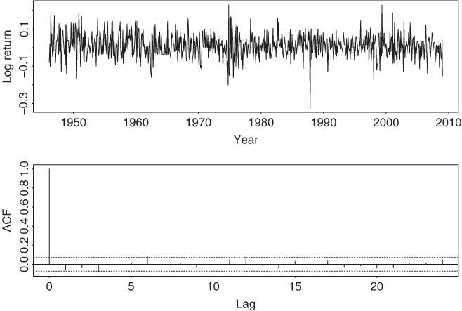
Table 2.5 Sample Extended Autocorrelation Function and a Simplified Table for the Monthly Log Returns of 3M Stock from February 1946 to December 2008

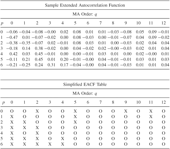
The simplified table exhibits a triangular pattern of O with its upper left vertex at the order (p, q) = (0, 0). A few exceptions of X appear when q = 2, 5, 9, and 11. However, the EACF table shows that the values of sample ACF corresponding to those X are around 0.08 or 0.09. These ACFs are only slightly greater than . Indeed, if 1% critical value is used, those X would become O in the simplified EACF table. Consequently, the EACF suggests that the monthly log returns of 3M stock follow an ARMA(0,0) model (i.e., a white noise series). This is in agreement with the result suggested by the sample ACF in Figure 2.9.

The information criteria discussed earlier can also be used to select ARMA(p, q) models. Typically, for some prespecified positive integers P and Q, one computes AIC (or BIC) for ARMA(p, q) models, where 0 ≤ p ≤ P and 0 ≤ q ≤ Q, and selects the model that gives the minimum AIC (or BIC). This approach requires maximum-likelihood estimation of many models and in some cases may encounter the difficulty of overfitting in estimation.

Once an ARMA(p, q) model is specified, its parameters can be estimated by either the conditional or exact-likelihood method. In addition, the Ljung–Box statistics of the residuals can be used to check the adequacy of a fitted model. If the model is correctly specified, then Q(m) follows asymptotically a chi-squared distribution with m − g degrees of freedom, where g denotes the number of AR or MA coefficients fitted in the model.

2.6.4 Forecasting Using an ARMA Model

Like the behavior of ACF, forecasts of an ARMA(p, q) model have similar characteristics as those of an AR(p) model after adjusting for the impacts of the MA component on the lower horizon forecasts. Denote the forecast origin by h and the available information by Fh. The 1-step-ahead forecast of rh+1 can be easily obtained from the model as

and the associated forecast error is . The variance of 1-step-ahead forecast error is Var[. For the ℓ-step-ahead forecast, we have

where it is understood that if ℓ − i ≤ 0 and ah(ℓ − i) = 0 if ℓ − i > 0 and ah(ℓ − i) = ah+ℓ−i if ℓ − i ≤ 0. Thus, the multistep-ahead forecasts of an ARMA model can be computed recursively. The associated forecast error is

which can be computed easily via a formula to be given in Eq. (2.34).

2.6.5 Three Model Representations for an ARMA Model

In this section, we briefly discuss three model representations for a stationary ARMA(p, q) model. The three representations serve three different purposes. Knowing these representations can lead to a better understanding of the model. The first representation is the ARMA(p, q) model in Eq. (2.28). This representation is compact and useful in parameter estimation. It is also useful in computing recursively multistep-ahead forecasts of rt; see the discussion in the last section.

For the other two representations, we use long division of two polynomials. Given two polynomials and , we can obtain, by long division, that

2.29

and

2.30

For instance, if ϕ(B) = 1 − ϕ1B and θ(B) = 1 − θ1B, then

From the definition, ψ(B)π(B) = 1. Making use of the fact that Bc = c for any constant (because the value of a constant is time invariant), we have

AR Representation

Using the result of long division in Eq. (2.30), the ARMA(p, q) model can be written as

2.31

This representation shows the dependence of the current return rt on the past returns rt−i, where i > 0. The coefficients {πi} are referred to as the π weights of an ARMA model. To show that the contribution of the lagged value rt−i to rt is diminishing as i increases, the πi coefficient should decay to zero as i increases. An ARMA(p, q) model that has this property is said to be invertible. For a pure AR model, θ(B) = 1 so that π(B) = ϕ(B), which is a finite-degree polynomial. Thus, πi = 0 for i > p, and the model is invertible. For other ARMA models, a sufficient condition for invertibility is that all the zeros of the polynomial θ(B) are greater than unity in modulus. For example, consider the MA(1) model rt = (1 − θ1B)at. The zero of the first-order polynomial 1 − θ1B is B = 1/θ1. Therefore, an MA(1) model is invertible if |1/θ1| > 1. This is equivalent to |θ1| < 1.

From the AR representation in Eq. (2.31), an invertible ARMA(p, q) series rt is a linear combination of the current shock at and a weighted average of the past values. The weights decay exponentially for more remote past values.

MA Representation

Again, using the result of long division in Eq. (2.29), an ARMA(p, q) model can also be written as

2.32

where μ = E(rt) = ϕ0/(1 − ϕ1 − ⋯ − ϕp). This representation shows explicitly the impact of the past shock at−i (i > 0) on the current return rt. The coefficients {ψi} are referred to as the impulse response function of the ARMA model. For a weakly stationary series, the ψi coefficients decay exponentially as i increases. This is understandable as the effect of shock at−i on the return rt should diminish over time. Thus, for a stationary ARMA model, the shock at−i does not have a permanent impact on the series. If ϕ0 ≠ 0, then the MA representation has a constant term, which is the mean of rt [i.e., ϕ0/(1 − ϕ1 − ⋯ − ϕp)].

The MA representation in Eq. (2.32) is also useful in computing the variance of a forecast error. At the forecast origin h, we have the shocks ah, ah−1, … . Therefore, the ℓ-step-ahead point forecast is

2.33

and the associated forecast error is

Consequently, the variance of ℓ-step-ahead forecast error is

2.34

which, as expected, is a nondecreasing function of the forecast horizon ℓ.

Finally, the MA representation in Eq. (2.32) provides a simple proof of mean reversion of a stationary time series. The stationarity implies that ψi approaches zero as i → ∞. Therefore, by Eq. (2.33), we have as ℓ → ∞. Because is the conditional expectation of rh+ℓ at the forecast origin h, the result says that in the long term the return series is expected to approach its mean, that is, the series is mean reverting. Furthermore, using the MA representation in Eq. (2.32), we have . Consequently, by Eq. (2.34), we have Var[eh(ℓ)] → Var(rt) as ℓ → ∞. The speed by which approaches μ determines the speed of mean reverting.