Example 10.7

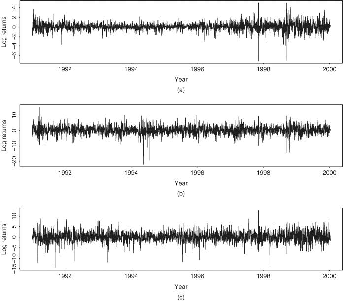
We demonstrate the proposed sequential procedure by building a volatility model for the daily log returns of the S&P 500 index and the stocks of Cisco Systems and Intel Corporation. The data span is from January 2, 1991, to December 31, 1999, with 2275 observations. The log returns are in percentages and shown in Figure 10.14. Components of the return series are ordered as . The sample means, standard errors, and correlation matrix of the data are

Figure 10.14 Time plots of daily log returns in percentages of (a) S&P 500 index and stocks of (b) Cisco Systems and (c) Intel Corporation from January 2, 1991, to December 31, 1999.

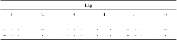
Using the Ljung–Box statistics to detect any serial dependence in the return series, we obtain Q3(1) = 26.20, Q3(4) = 79.73, and Q3(8) = 123.68. These test statistics are highly significant with p values close to zero as compared with chi-squared distributions with degrees of freedom 9, 36, and 72, respectively. There is indeed some serial dependence in the data. Table 10.3 gives the first five lags of sample cross-correlation matrices shown in the simplified notation of Chapter 8. An examination of the table shows that (a) the daily log returns of the S&P 500 index does not depend on the past returns of Cisco or Intel, (b) the log return of Cisco stock has some serial correlations and depends on the past returns of the S&P 500 index (see lags 2 and 5), and (c) the log return of Intel stock depends on the past returns of the S&P 500 index (see lags 1 and 5). These observations are similar to those between the returns of IBM stock and the S&P 500 index analyzed in Chapter 8. They suggest that returns of individual large-cap companies tend to be affected by the past behavior of the market. However, the market return is not significantly affected by the past returns of individual companies.

Table 10.3 Sample Cross-Correlation Matrices of Daily Log Returns of S&P 500 Index and Stocks of Cisco Systems and Intel Corporation from January 2, 1991, to December 31, 1999

Turning to volatility modeling and following the suggested procedure, we start with the log returns of the S&P 500 index and obtain the model

10.33

where standard errors of the parameters in the mean equation are 0.016, 0.023, 0.020, 0.022, and 0.020, respectively, and those of the parameters in the volatility equation are 0.002, 0.006, and 0.007, respectively. Univariate Ljung–Box statistics of the standardized residuals and their squared series fail to detect any remaining serial correlation or conditional heteroscedasticity in the data. Indeed, we have Q(10) = 7.38(0.69) for the standardized residuals and Q(10) = 3.14(0.98) for the squared series.

Augmenting the daily log returns of Cisco stock to the system, we build a bivariate model with mean equations given by

10.34

where all of the estimates are statistically significant at the 1% level. Using the notation of Cholesky decomposition, we obtain the volatility equations as

10.35

where b1t = a1t, b2t = a2t − q21, tb1t, standard errors of the parameters in the equation of g11, t are 0.001, 0.005, and 0.006, those of the parameters in the equation of q21, t are 0.156, 0.099, and 0.011, and those of the parameters in the equation of g22, t are 0.029, 0.008, and 0.011, respectively. The bivariate Ljung–Box statistics of the standardized residuals fail to detect any remaining serial dependence or conditional heteroscedasticity. The bivariate model is adequate. Comparing with Eq. (10.33), we see that the difference between the marginal and univariate models of r1t is small.

The next and final step is to augment the daily log returns of Intel stock to the system. The mean equations become

10.36

where standard errors of the parameters in the first equation are 0.016 and 0.017, those of the parameters in the second equation are 0.052, 0.059, and 0.021, and those of the parameters in the third equation are 0.050, 0.057, and 0.022, respectively. All estimates are statistically significant at about the 1% level. As expected, the mean equations for r1t and r2t are essentially the same as those in the bivariate case.

The three-dimensional time-varying volatility model becomes a bit more complicated, but it remains manageable as

10.37

where b1t = a1t, b2t = a2t − q21, tb1t, b3t = a3t − q31, tb1t − q32, tb2t, and standard errors of the parameters are given in Table 10.4. Except for the constant term of the q32, t equation, all estimates are significant at the 5% level. Let be the standardized residual series, where is the fitted conditional standard error of the ith return. The Ljung–Box statistics of give Q3(4) = 34.48(0.31) and Q3(8) = 60.42(0.70), where the degrees of freedom of the chi-squared distributions are 31 and 67, respectively, after adjusting for the number of parameters used in the mean equations. For the squared standardized residual series , we have and . Therefore, the fitted model appears to be adequate in modeling the conditional means and volatilities.

Table 10.4 Standard Errors of Parameter Estimates of Three-Dimensional Volatility Model for Daily Log Returns in Percentages of S&P 500 Index and Stocks of Cisco Systems and Intel Corporation from January 2, 1991, to December 31, 1999a

a 
  The ordering of the parameter is the same as appears in Eq. (10.37).

The three-dimensional volatility model in Eq. (10.37) shows some interesting features. First, it is essentially a time-varying correlation GARCH(1,1) model because only lag-1 variables are used in the equations. Second, the volatility of the daily log returns of the S&P 500 index does not depend on the past volatilities of Cisco or Intel stock returns. Third, by taking the inverse transformation of the Cholesky decomposition, the volatilities of daily log returns of Cisco and Intel stocks depend on the past volatility of the market return; see the relationships between elements of , , and given in Section 10.3. Fourth, the correlation quantities qij, t have high persistence with large AR(1) coefficients.

Figure 10.15 shows the fitted volatility processes of the model (i.e., ) for the data. The volatility of the index return is much smaller than those of the two individual stock returns. The plots also show that the volatility of the index return has increased in recent years, but this is not the case for the return of Cisco Systems. Figure 10.16 shows the time-varying correlation coefficients between the three return series. Of particular interest is to compare Figures 10.15 and 10.16. They show that the correlation coefficient between two return series increases when the returns are volatile. This is in agreement with the empirical study of relationships between international stock market indexes for which the correlation between two markets tends to increase during a financial crisis.

Figure 10.15 Time plots of fitted volatilities for daily log returns, in percentages, of (a) S&P 500 index and stocks of (b) Cisco Systems and (c) Intel Corporation from January 2, 1991, to December 31, 1999.

Figure 10.16 Time plots of fitted time-varying correlation coefficients between daily log returns of S&P 500 index and stocks of Cisco Systems and Intel Corporation from January 2, 1991, to December 31, 1999.

The volatility model in Eq. (10.37) consists of two sets of equations. The first set of equations describes the time evolution of conditional variances (i.e., gii, t), and the second set of equations deals with correlation coefficients (i.e., qij, t with i > j). For this particular data set, an AR(1) model might be sufficient for the correlation equations. Similarly, a simple AR model might also be sufficient for the conditional variances. Define , where vii, t = ln(gii, t), and . The previous discussion suggests that we can use the simple lag-1 models

as exact functions to model the volatility of asset returns, where are constant vectors and are 3 × 3 real-valued matrices. If a noise term is also included in the above equations, then the models become

where are random shocks with mean zero and a positive-definite covariance matrix, and we have a simple multivariate stochastic volatility model. In a recent manuscript, Chib, Nardari, and Shephard (1999) use Markov chain Monte Carlo (MCMC) methods to study high-dimensional stochastic volatility models. The model considered there allows for time-varying correlations, but in a relatively restrictive manner. Additional references of multivariate volatility model include Harvey, Ruiz, and Shephard (1994). We discuss MCMC methods in volatility modeling in Chapter 12.