Example 10.8

Consider again the monthly log returns, in percentages, of IBM stock and the S&P 500 index of Example 10.5. Using the bivariate AR(3) model of Example 8.4, we obtain an innovational series . Performing a PCA on based on its covariance matrix, we obtained eigenvalues 63.373 and 13.489. The first eigenvalue explains 82.2% of the generalized variance of . Therefore, we may choose the first principal component xt = 0.797a1t + 0.604a2t as the common factor. Alternatively, as shown by the model in Example 8.4, the serial dependence in is weak and, hence, one can perform the PCA on directly. For this particular instance, the two eigenvalues of the sample covariance matrix of are 63.625 and 13.513, which are essentially the same as those based on . The first principal component explains approximately 82.5% of the generalized variance of , and the corresponding common factor is xt = 0.796r1t + 0.605r2t. Consequently, for the two monthly log return series considered, the effect of the conditional mean equations on PCA is negligible.

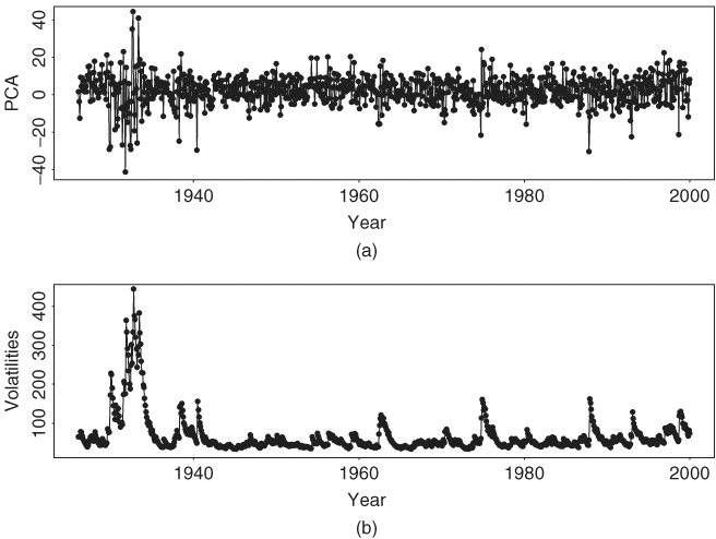
Based on the prior discussion and for simplicity, we use xt = 0.796r1t + 0.605r2t as a common factor for the two monthly return series. Figure 10.17(a) shows the time plot of this common factor. If univariate Gaussian GARCH models are entertained, we obtain the following model for xt:

10.38

All parameter estimates of the previous model are highly significant at the 1% level, and the Ljung–Box statistics of the standardized residuals and their squared series fail to detect any model inadequacy. Figure 10.17(b) shows the fitted volatility of xt [i.e., the sample series in Eq. (10.38)].

Figure 10.17 (a) Time plot of first principal component of monthly log returns of IBM stock and S&P 500 index. (b) Fitted volatility process based on a GARCH(1,1) model.

Using of model (10.38) as a common volatility factor, we obtain the following model for the original monthly log returns. The mean equations are

where standard errors of the parameters in the first equation are 0.211, 0.030, 0.031, and 0.043, respectively, and standard error of the parameter in the second equation is 0.165. The conditional variance equation is

10.39

where, as before, standard errors are in parentheses, and is obtained from model (10.38). The conditional correlation equation is

10.40

where standard errors of the three parameters are 0.025, 0.038, and 0.015, respectively. Defining the standardized residuals as before, we obtain Q2(4) = 15.37(0.29) and Q2(8) = 34.24(0.23), where the number in parentheses denotes the p value. Therefore, the standardized residuals have no serial correlations. Yet we have and for the squared standardized residuals. The volatility model in Eq. (10.39) does not adequately handle the conditional heteroscedasticity of the data especially at higher lags. This is not surprising as the single common factor only explains about 82.5% of the generalized variance of the data.

Comparing the factor model in Eqs. (10.39) and (10.40) with the time-varying correlation model in Eqs. (10.26) and (10.27), we see that (a) the correlation equations of the two models are essentially the same, (b) as expected the factor model uses fewer parameters in the volatility equation, and (c) the common-factor model provides a reasonable approximation to the volatility process of the data.

Remark

In Example 10.8, we used a two-step estimation procedure. In the first step, a volatility model is built for the common factor. The estimated volatility is treated as given in the second step to estimate the multivariate volatility model. Such an estimation procedure is simple but may not be efficient. A more efficient estimation procedure is to perform a joint estimation. This can be done relatively easily provided that the common factors are known. For example, for the monthly log returns of Example 10.8, a joint estimation of Eqs. (10.38)–(10.40) can be performed if the common factor xt = 0.769r1t + 0.605r2t is treated as given.