8.7 Threshold Cointegration and Arbitrage

In this section, we focus on detecting arbitrage opportunities in index trading by using multivariate time series methods. We also demonstrate that simple univariate nonlinear models of Chapter 4. can be extended naturally to the multivariate case in conjunction with the idea of cointegration.

Our study considers the relationship between the price of the S&P 500 index futures and the price of the shares underlying the index on the cash market. Let ft, ℓ be the log price of the index futures at time t with maturity ℓ, and let st be the log price of the shares underlying the index on the cash market at time t. A version of the cost-of-carry model in the finance literature states

8.43

where rt, ℓ is the risk-free interest rate, qt, ℓ is the dividend yield with respect to the cash price at time t, and (ℓ − t) is the time to maturity of the futures contract; see Brenner and Kroner (1995), Dwyer, Locke, and Yu (1996), and the references therein.

The process of model (8.43) must be unit-root stationary; otherwise there exist persistent arbitrage opportunities. Here an arbitrage trading consists of simultaneously buying (short-selling) the security index and selling (buying) the index futures whenever the log prices diverge by more than the cost of carrying the index over time until maturity of the futures contract. Under the weak stationarity of , for arbitrage to be profitable, must exceed a certain value in modulus determined by transaction costs and other economic and risk factors.

It is commonly believed that the ft, ℓ and st series of the S&P 500 index contain a unit root, but Eq. (8.43) indicates that they are cointegrated after adjusting for the effect of interest rate and dividend yield. The cointegrating vector is (1, − 1) after the adjustment, and the cointegrated series is . Therefore, one should use an error correction form to model the return series , where Δft = ft, ℓ − ft−1, ℓ and Δst = st − st−1, where for ease in notation we drop the maturity time ℓ from the subscript of Δft.  □

8.7.1 Multivariate Threshold Model

In practice, arbitrage tradings affect the dynamic of the market, and hence the model for may vary over time depending on the presence or absence of arbitrage tradings. Consequently, the prior discussions lead naturally to the following model:

8.44

where , γ1 < 0 < γ2 are two real numbers, and are sequences of two-dimensional white noises and are independent of each other. Here we use because the actual value of is relatively small.

The model in Eq. (8.44) is referred to as a multivariate threshold model with three regimes. The two real numbers γ1 and γ2 are the thresholds and zt−1 is the threshold variable. The threshold variable zt−1 is supported by the data; see Tsay (1998). In general, one can select zt−d as a threshold variable by considering d ∈ {1, … , d0}, where d0 is a prespecified positive integer.

Model (8.44) is a generalization of the threshold autoregressive model of Chapter 4. It is also a generalization of the error correlation model of Eq. (8.36). As mentioned earlier, an arbitrage trading is profitable only when or, equivalently, zt is large in modulus. Therefore, arbitrage tradings only occurred in regimes 1 and 3 of model (8.44). As such, the dynamic relationship between ft, ℓ and st in regime 2 is determined mainly by the normal market force, and hence the two series behave more or less like a random walk. In other words, the two log prices in the middle regime should be free from arbitrage effects and, hence, free from the cointegration constraint. From an econometric viewpoint, this means that the estimate of in the middle regime should be insignificant.

In summary, we expect that the cointegration effects between the log price of the futures and the log price of security index on the cash market are significant in regimes 1 and 3, but insignificant in regime 2. This phenomenon is referred to as a threshold cointegration; see Balke and Fomby (1997).

8.7.2 The Data

The data used in this case study are the intraday transaction data of the S&P 500 index in May 1993 and its June futures contract traded at the Chicago Mercantile Exchange; see Forbes, Kalb, and Kofman (1999), who used the data to construct a minute-by-minute bivariate price series with 7060 observations. To avoid the undue influence of unusual returns, I replaced 10 extreme values (5 on each side) by the simple average of their two nearest neighbors. This step does not affect the qualitative conclusion of the analysis but may affect the conditional heteroscedasticity in the data. For simplicity, we do not consider conditional heteroscedasticity in the study. Figure 8.16 shows the time plots of the log returns of the index futures and cash prices and the associated threshold variable zt = of model (8.43).

Figure 8.16 Time plots of 1-minute log returns of S&P 500 index futures and cash prices and associated threshold variable in May 1993: (a) log returns of index futures, (b) log returns of index cash prices, and (c) zt series.

8.7.3 Estimation

A formal specification of the multivariate threshold model in Eq. (8.44) includes selecting the threshold variable, determining the number of regimes, and choosing the order p for each regime. Interested readers are referred to Tsay (1998) and Forbes, Kalb, and Kofman (1999). The thresholds γ1 and γ2 can be estimated by using some information criteria [e.g., the Akaike information criterion (AIC) or the sum of squares of residuals]. Assuming p = 8, d ∈ {1, 2, 3, 4}, γ1 ∈ [ − 0.15, − 0.02], and γ2 ∈ [0.025, 0.145], and using a grid search method with 300 points on each of the two intervals, the AIC selects zt−1 as the threshold variable with thresholds and . Details of the parameter estimates are given in Table 8.8.

Table 8.8 Least-Squares Estimates and Their t Ratios of Multivariate Threshold Model in Eq. (8.43) for S&P 500 Index Data in May 1993a

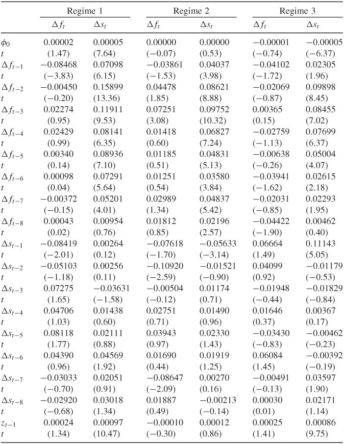
aThe numbers of data points for the three regimes are 2234, 2410, and 2408, respectively.

From Table 8.8, we make the following observations. First, the t ratios of in the middle regime show that, as expected, the estimates are insignificant at the 5% level, confirming that there is no cointegration between the two log prices in the absence of arbitrage opportunities. Second, Δft depends negatively on Δft−1 in all three regimes. This is in agreement with the bid–ask bounce discussed in Chapter 5. Third, past log returns of the index futures seem to be more informative than the past log returns of the cash prices because there are more significant t ratios in Δft−i than in Δst−i. This is reasonable because futures series are in general more liquid. For more information on index arbitrage, see Dwyer, Locke, and Yu (1996).