
To better understand cointegration, we focus on VAR models for their simplicity in estimation. Consider a k-dimensional VAR(p) time series ![]() with possible time trend so that the model is
with possible time trend so that the model is
8.35 ![]()
where the innovation ![]() is assumed to be Gaussian and
is assumed to be Gaussian and ![]() =
= ![]() , where
, where ![]() and
and ![]() are k-dimensional constant vectors. Write
are k-dimensional constant vectors. Write ![]() =
= ![]() . Recall that if all zeros of the determinant
. Recall that if all zeros of the determinant ![]() are outside the unit circle, then
are outside the unit circle, then ![]() is unit-root stationary. In the literature, a unit-root stationary series is said to be an I(0) process; that is, it is not integrated. If
is unit-root stationary. In the literature, a unit-root stationary series is said to be an I(0) process; that is, it is not integrated. If ![]() = 0, then
= 0, then ![]() is unit-root nonstationary. For simplicity, we assume that
is unit-root nonstationary. For simplicity, we assume that ![]() is at most an integrated process of order 1; that is, an I(1) process. This means that (1 − B)xit is unit-root stationary if xit itself is not.
is at most an integrated process of order 1; that is, an I(1) process. This means that (1 − B)xit is unit-root stationary if xit itself is not.
An error correction model (ECM) for the VAR(p) process ![]() is
is
where ![]() are defined in Eq. (8.34) and
are defined in Eq. (8.34) and ![]() =
= ![]() . We refer to the term
. We refer to the term ![]() of Eq. (8.36) as the error correction term, which plays a key role in cointegration study. Notice that
of Eq. (8.36) as the error correction term, which plays a key role in cointegration study. Notice that ![]() can be recovered from the ECM representation via
can be recovered from the ECM representation via
![]()
where ![]() , the zero matrix. Based on the assumption that
, the zero matrix. Based on the assumption that ![]() is at most I(1),
is at most I(1), ![]() of Eq. (8.36) is an I(0) process.
of Eq. (8.36) is an I(0) process.
If ![]() contains unit roots, then
contains unit roots, then ![]() = 0 so that
= 0 so that ![]() is singular. Therefore, three cases are of interest in considering the ECM in Eq. (8.36):
is singular. Therefore, three cases are of interest in considering the ECM in Eq. (8.36):
1. Rank(![]() ) = 0. This implies
) = 0. This implies ![]() and
and ![]() is not cointegrated. The ECM of Eq. (8.36) reduces to
is not cointegrated. The ECM of Eq. (8.36) reduces to
![]()
so that ![]() follows a VAR(p − 1) model with deterministic trend
follows a VAR(p − 1) model with deterministic trend ![]() .
.
2. Rank(![]() ) = k. This implies that
) = k. This implies that ![]() and
and ![]() contains no unit roots; that is,
contains no unit roots; that is, ![]() is I(0). The ECM model is not informative and one studies
is I(0). The ECM model is not informative and one studies ![]() directly.
directly.
3. ![]() . In this case, one can write
. In this case, one can write ![]() as
as
where ![]() and
and ![]() are k × m matrices with Rank(
are k × m matrices with Rank(![]() ) = Rank(
) = Rank(![]() ) = m. The ECM of Eq. (8.36) becomes
) = m. The ECM of Eq. (8.36) becomes
8.38 ![]()
This means that ![]() is cointegrated with m linearly independent cointegrating vectors,
is cointegrated with m linearly independent cointegrating vectors, ![]() , and has k − m unit roots that give k − m common stochastic trends of
, and has k − m unit roots that give k − m common stochastic trends of ![]() .
.
If ![]() is cointegrated with Rank(
is cointegrated with Rank(![]() ) = m, then a simple way to obtain a presentation of the k − m common trends is to obtain an orthogonal complement matrix
) = m, then a simple way to obtain a presentation of the k − m common trends is to obtain an orthogonal complement matrix ![]() of
of ![]() ; that is,
; that is, ![]() is a k × (k − m) matrix such that
is a k × (k − m) matrix such that ![]() , a (k − m) × m zero matrix, and use
, a (k − m) × m zero matrix, and use ![]() . To see this, one can premultiply the ECM by
. To see this, one can premultiply the ECM by ![]() and use
and use ![]() to see that there would be no error correction term in the resulting equation. Consequently, the (k − m)-dimensional series
to see that there would be no error correction term in the resulting equation. Consequently, the (k − m)-dimensional series ![]() should have k − m unit roots. For illustration, consider the bivariate example of Section 8.5.1. For this special series,
should have k − m unit roots. For illustration, consider the bivariate example of Section 8.5.1. For this special series, ![]() and
and ![]() . Therefore,
. Therefore, ![]() , which is precisely the unit-root nonstationary series y1t in Eq. (8.32).
, which is precisely the unit-root nonstationary series y1t in Eq. (8.32).
Note that the factorization in Eq. (8.37) is not unique because for any m × m orthogonal matrix ![]() satisfying
satisfying ![]() , we have a
, we have a
![]()
where both ![]() and
and ![]() are also of rank m. Additional constraints are needed to uniquely identify
are also of rank m. Additional constraints are needed to uniquely identify ![]() and
and ![]() . It is common to require that
. It is common to require that ![]() , where
, where ![]() is the m × m identity matrix and
is the m × m identity matrix and ![]() is a (k − m) × m matrix. In practice, this may require reordering of the elements of
is a (k − m) × m matrix. In practice, this may require reordering of the elements of ![]() such that the first m components all have a unit root. The elements of
such that the first m components all have a unit root. The elements of ![]() and
and ![]() must also satisfy other constraints for the process
must also satisfy other constraints for the process ![]() to be unit-root stationary. For example, consider the case of a bivariate VAR(1) model with one cointegrating vector. Here k = 2, m = 1, and the ECM is
to be unit-root stationary. For example, consider the case of a bivariate VAR(1) model with one cointegrating vector. Here k = 2, m = 1, and the ECM is
![]()
Premultiplying the prior equation by ![]() , using
, using ![]() , and moving wt−1 to the right-hand side of the equation, we obtain
, and moving wt−1 to the right-hand side of the equation, we obtain
![]()
where ![]() . This implies that wt is a stationary AR(1) process. Consequently, αi and β1 must satisfy the stationarity constraint |1 + α1 + α2β1| < 1.
. This implies that wt is a stationary AR(1) process. Consequently, αi and β1 must satisfy the stationarity constraint |1 + α1 + α2β1| < 1.
The prior discussion shows that the rank of ![]() in the ECM of Eq. (8.36) is the number of cointegrating vectors. Thus, to test for cointegration, one can examine the rank of
in the ECM of Eq. (8.36) is the number of cointegrating vectors. Thus, to test for cointegration, one can examine the rank of ![]() . This is the approach taken by Johansen (1988, 1995) and Reinsel and Ahn (1992).
. This is the approach taken by Johansen (1988, 1995) and Reinsel and Ahn (1992).
8.6.1 Specification of the Deterministic Function
Similar to the univariate case, the limiting distributions of cointegration tests depend on the deterministic function ![]() . In this section, we discuss some specifications of
. In this section, we discuss some specifications of ![]() that have been proposed in the literature. To understand some of the statements made below, keep in mind that
that have been proposed in the literature. To understand some of the statements made below, keep in mind that ![]() provides a presentation for the common stochastic trends of
provides a presentation for the common stochastic trends of ![]() if it is cointegrated.
if it is cointegrated.
1. ![]() : In this case, all the component series of
: In this case, all the component series of ![]() are I(1) without drift and the stationary series
are I(1) without drift and the stationary series ![]() has mean zero.
has mean zero.
2. ![]() , where
, where ![]() is an m-dimensional nonzero constant vector. The ECM becomes
is an m-dimensional nonzero constant vector. The ECM becomes
![]()
so that the components of ![]() are I(1) without drift, but
are I(1) without drift, but ![]() have a nonzero mean
have a nonzero mean ![]() . This is referred to as the case of restricted constant.
. This is referred to as the case of restricted constant.
3. ![]() , which is nonzero. Here the component series of
, which is nonzero. Here the component series of ![]() are I(1) with drift
are I(1) with drift ![]() and
and ![]() may have a nonzero mean.
may have a nonzero mean.
4. ![]() , where
, where ![]() is a nonzero vector. The ECM becomes
is a nonzero vector. The ECM becomes
![]()
so that the components of ![]() are I(1) with drift
are I(1) with drift ![]() and
and ![]() has a linear time trend related to
has a linear time trend related to ![]() . This is the case of restricted trend.
. This is the case of restricted trend.
5. ![]() =
= ![]() , where
, where ![]() are nonzero. Here both the constant and trend are unrestricted. The components of
are nonzero. Here both the constant and trend are unrestricted. The components of ![]() are I(1) and have a quadratic time trend and
are I(1) and have a quadratic time trend and ![]() have a linear trend.
have a linear trend.
Obviously, the last case is not common in empirical work. The first case is not common for economic time series but may represent the log price series of some assets. The third case is also useful in modeling asset prices.
8.6.2 Maximum-Likelihood Estimation
In this section, we briefly outline the maximum-likelihood estimation (MLE) of a cointegrated VAR(p) model. Suppose that the data are ![]() . Without loss of generality, we write
. Without loss of generality, we write ![]() , where
, where ![]() , and it is understood that
, and it is understood that ![]() depends on the specification of the previous section. For a given m, which is the rank of
depends on the specification of the previous section. For a given m, which is the rank of ![]() , the ECM model becomes
, the ECM model becomes
8.39 ![]()
where t = p + 1, … , T. A key step in the estimation is to concentrate the likelihood function with respect to the deterministic term and the stationary effects. This is done by considering the following two multivariate linear regressions:
Let ![]() and
and ![]() be the residuals of Eqs. (8.40) and (8.41), respectively. Define the sample covariance matrices
be the residuals of Eqs. (8.40) and (8.41), respectively. Define the sample covariance matrices
![]()
Next, compute the eigenvalues and eigenvectors of ![]() with respect to
with respect to ![]() . This amounts to solving the eigenvalue problem
. This amounts to solving the eigenvalue problem
![]()
Denote the eigenvalue and eigenvector pairs by ![]() , where
, where ![]() . Here the eigenvectors are normalized so that
. Here the eigenvectors are normalized so that ![]() , where
, where ![]() is the matrix of eigenvectors.
is the matrix of eigenvectors.
The unnormalized MLE of the cointegrating vector ![]() is
is ![]() and from which we can obtain an MLE for
and from which we can obtain an MLE for ![]() that satisfies the identifying constraint and normalization condition. Denote the resulting estimate by
that satisfies the identifying constraint and normalization condition. Denote the resulting estimate by ![]() with the subscript c signifying constraints. The MLE of other parameters can then be obtained by the multivariate linear regression
with the subscript c signifying constraints. The MLE of other parameters can then be obtained by the multivariate linear regression
![]()
The maximized value of the likelihood function based on m cointegrating vectors is
![]()
This value is used in the maximum-likelihood ratio test for testing Rank(![]() ) = m. Finally, estimates of the orthogonal complements of
) = m. Finally, estimates of the orthogonal complements of ![]() and
and ![]() can be obtained using
can be obtained using
![]()
8.6.3 Cointegration Test
For a specified deterministic term ![]() , we now discuss the maximum-likelihood test for testing the rank of the
, we now discuss the maximum-likelihood test for testing the rank of the ![]() matrix in Eq. (8.36). Let H(m) be the null hypothesis that the rank of
matrix in Eq. (8.36). Let H(m) be the null hypothesis that the rank of ![]() is m. For example, under H(0), Rank(
is m. For example, under H(0), Rank(![]() ) = 0 so that
) = 0 so that ![]() and there is no cointegration. The hypotheses of interest are
and there is no cointegration. The hypotheses of interest are
![]()
For testing purpose, the ECM in Eq. (8.36) becomes
![]()
where t = p + 1, … , T. Our goal is to test the rank of ![]() . Mathematically, the rank of
. Mathematically, the rank of ![]() is the number of nonzero eigenvalues of
is the number of nonzero eigenvalues of ![]() , which can be obtained if a consistent estimate of
, which can be obtained if a consistent estimate of ![]() is available. Based on the prior equation, which is in the form of a multivariate linear regression, we see that
is available. Based on the prior equation, which is in the form of a multivariate linear regression, we see that ![]() is related to the covariance matrix between
is related to the covariance matrix between ![]() and
and ![]() after adjusting for the effects of
after adjusting for the effects of ![]() and
and ![]() for i = 1, … , p − 1. The necessary adjustments can be achieved by the techniques of multivariate linear regression shown in the previous section. Indeed, the adjusted series of
for i = 1, … , p − 1. The necessary adjustments can be achieved by the techniques of multivariate linear regression shown in the previous section. Indeed, the adjusted series of ![]() and
and ![]() are
are ![]() and
and ![]() , respectively. The equation of interest for the cointegration test then becomes
, respectively. The equation of interest for the cointegration test then becomes
![]()
Under the normality assumption, the likelihood ratio test for testing the rank of ![]() in the prior equation can be done by using the canonical correlation analysis between
in the prior equation can be done by using the canonical correlation analysis between ![]() and
and ![]() . See Johnson and Wichern (1998) for information on canonical correlation analysis. The associated canonical correlations are the partial canonical correlations between
. See Johnson and Wichern (1998) for information on canonical correlation analysis. The associated canonical correlations are the partial canonical correlations between ![]() and
and ![]() because the effects of
because the effects of ![]() and
and ![]() have been adjusted. The quantities
have been adjusted. The quantities ![]() are the squared canonical correlations between
are the squared canonical correlations between ![]() and
and ![]() .
.
Consider the hypotheses
![]()
Johansen (1988) proposes the likelihood ratio (LR) statistic
8.42 ![]()
to perform the test. If Rank(![]() ) = m, then
) = m, then ![]() should be small for i > m and hence LRtr(m) should be small. This test is referred to as the trace cointegration test. Due the presence of unit roots, the asymptotic distribution of LRtr(m) is not chi squared but a function of standard Brownian motions. Thus, critical values of LRtr(m) must be obtained via simulation.
should be small for i > m and hence LRtr(m) should be small. This test is referred to as the trace cointegration test. Due the presence of unit roots, the asymptotic distribution of LRtr(m) is not chi squared but a function of standard Brownian motions. Thus, critical values of LRtr(m) must be obtained via simulation.
Johansen (1988) also considers a sequential procedure to determine the number of cointegrating vectors. Specifically, the hypotheses of interest are
![]()
The LR ratio test statistic, called the maximum eigenvalue statistic, is
![]()
Again, critical values of the test statistics are nonstandard and must be evaluated via simulation.
8.6.4 Forecasting of Cointegrated VAR Models
The fitted ECM can be used to produce forecasts. First, conditioned on the estimated parameters, the ECM equation can be used to produce forecasts of the differenced series ![]() . Such forecasts can in turn be used to obtain forecasts of
. Such forecasts can in turn be used to obtain forecasts of ![]() . A difference between ECM forecasts and the traditional VAR forecasts is that the ECM approach imposes the cointegration relationships in producing the forecasts.
. A difference between ECM forecasts and the traditional VAR forecasts is that the ECM approach imposes the cointegration relationships in producing the forecasts.
8.6.5 An Example
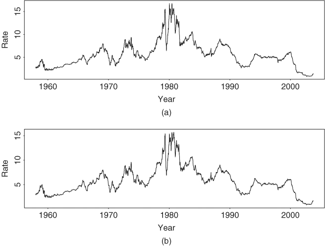
To demonstrate the analysis of cointegrated VAR models, we consider two weekly U.S. short-term interest rates. The series are the 3-month Treasury bill (TB) rate and 6-month Treasury bill rate from December 12, 1958, to August 6, 2004, for 2383 observations. The TB rates are from the secondary market and obtained from the Federal Reserve Bank of St. Loius. Figure 8.12 shows the time plots of the interest rates. As expected, the two series move closely together.
Figure 8.12 Time plots of weekly U.S. interest rate from December 12, 1958, to August 6, 2004. (a) The 3-month Treasury bill rate and (b) 6-month Treasury bill rate. Rates are from secondary market.
Our analysis uses the S-Plus software with commands VAR for VAR analysis, coint for cointegration test, and VECM for vector error correction estimation. Denote the two series by tb3m and tb6m and define the vector series ![]() . The augmented Dickey–Fuller unit-root tests fail to reject the hypothesis of a unit root in the individual series; see Chapter 2. Indeed, the test statistics are − 2.34 and − 2.33 with p value about 0.16 for the 3-month and 6-month interest rate when an AR(3) model is used. Thus, we proceed to VAR modeling.
. The augmented Dickey–Fuller unit-root tests fail to reject the hypothesis of a unit root in the individual series; see Chapter 2. Indeed, the test statistics are − 2.34 and − 2.33 with p value about 0.16 for the 3-month and 6-month interest rate when an AR(3) model is used. Thus, we proceed to VAR modeling.
For the bivariate series ![]() , the BIC criterion selects a VAR(3) model:
, the BIC criterion selects a VAR(3) model:
> x=cbind(tb3m,tb6m)
> y=data.frame(x)
> ord.choice$ar.order
[1] 3
To perform a cointegration test, we choose a restricted constant for ![]() because there is no reason a priori to believe the existence of a drift in the U.S. interest rate. Both Johansen's tests confirm that the two series are cointegrated with one cointegrating vector when a VAR(3) model is entertained.
because there is no reason a priori to believe the existence of a drift in the U.S. interest rate. Both Johansen's tests confirm that the two series are cointegrated with one cointegrating vector when a VAR(3) model is entertained.
> cointst.rc=coint(x,trend=‘rc’, lags=2) % lags = p-1.
> cointst.rc
Call:
coint(Y = x, lags = 2, trend = “rc”)
Trend Specification:
H1*(r): Restricted constant
Trace tests sign. at the 5% level are flagged by ‘ +’.
Trace tests sign. at the 1% level are flagged by ‘++’.
Max Eig. tests sign. at the 5% level are flagged by ‘ *’.
Max Eig. tests sign. at the 1% level are flagged by ‘**’.
Tests for Cointegration Rank:
Eigenvalue Trace Stat 95% CV 99% CV
H(0)++** 0.0322 83.2712 19.96 24.60
H(1) 0.0023 5.4936 9.24 12.97
Max Stat 95% CV 99% CV
H(0)++** 77.7776 15.67 20.20
H(1) 5.4936 9.24 12.97
Next, we perform the maximum-likelihood estimation of the specified cointegrated VAR(3) model using an ECM presentation. The results are as follows:
> vecm.fit=VECM(cointst.rc)
> summary(vecm.fit)
Call:
VECM(test = cointst.rc)
Cointegrating Vectors:
coint.1
1.0000
tb6m −1.0124
(std.err) 0.0086
(t.stat) −118.2799
Intercept* 0.2254
(std.err) 0.0545
(t.stat) 4.1382
VECM Coefficients:
tb3m tb6m
coint.1 −0.0949 −0.0211
(std.err) 0.0199 0.0179
(t.stat) −4.7590 −1.1775
tb3m.lag1 0.0466 −0.0419
(std.err) 0.0480 0.0432
(t.stat) 0.9696 −0.9699
tb6m.lag1 0.2650 0.3164
(std.err) 0.0538 0.0484
(t.stat) 4.9263 6.5385
tb3m.lag2 −0.2067 −0.0346
(std.err) 0.0481 0.0433
(t.stat) −4.2984 −0.8005
tb6m.lag2 0.2547 0.0994
(std.err) 0.0543 0.0488
(t.stat) 4.6936 2.0356
Regression Diagnostics:
tb3m tb6m
R-squared 0.1081 0.0913
Adj. R-squared 0.1066 0.0898
Resid. Scale 0.2009 0.1807
> plot(vecm.fit)
Make a plot selection (or 0 to exit):
1: plot: All
2: plot: Response and Fitted Values
3: plot: Residuals
...
13: plot: PACF of Squared Cointegrating Residuals
Selection:
As expected, the output shows that the stationary series is wt ≈ tb3mt − tb6mt and the mean of wt is about − 0.225. The fitted ECM is
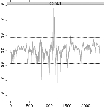
and the estimated standard errors of ait are 0.20 and 0.18, respectively. Adequacy of the fitted ECM can be examined via various plots. For illustration, Figure 8.13 shows the cointegrating residuals. Some large residuals are shown in the plot, which occurred in the early 1980s when the interest rates were high and volatile.
Figure 8.13 Time plot of cointegrating residuals for an ECM fit to weekly U.S. interest rate series. Data span is from December 12, 1958, to August 6, 2004.
Finally, we use the fitted ECM to produce 1-step- to 10-step-ahead forecasts for both ![]() and
and ![]() . The forecast origin is August 6, 2004.
. The forecast origin is August 6, 2004.
> vecm.fst=predict(vecm.fit, n.predict=10)
> summary(vecm.fst)
Predicted Values with Standard Errors:
tb3m tb6m
1-step-ahead −0.0378 −0.0642
(std.err) 0.2009 0.1807
2-step-ahead −0.0870 −0.0864
(std.err) 0.3222 0.2927
...
10-step-ahead −0.2276 −0.1314
(std.err) 0.8460 0.8157
> plot(vecm.fst,xold=diff(x),n.old=12)
> vecm.fit.level=VECM(cointst.rc,levels=T)
> vecm.fst.level=predict(vecm.fit.level, n.predict=10)
> summary(vecm.fst.level)
Predicted Values with Standard Errors:
tb3m tb6m
1-step-ahead 1.4501 1.7057
(std.err) 0.2009 0.1807
2-step-ahead 1.4420 1.7017
(std.err) 0.3222 0.2927
...
10-step-ahead 1.4722 1.7078
(std.err) 0.8460 0.8157
> plot(vecm.fst.level, xold=x, n.old=50)
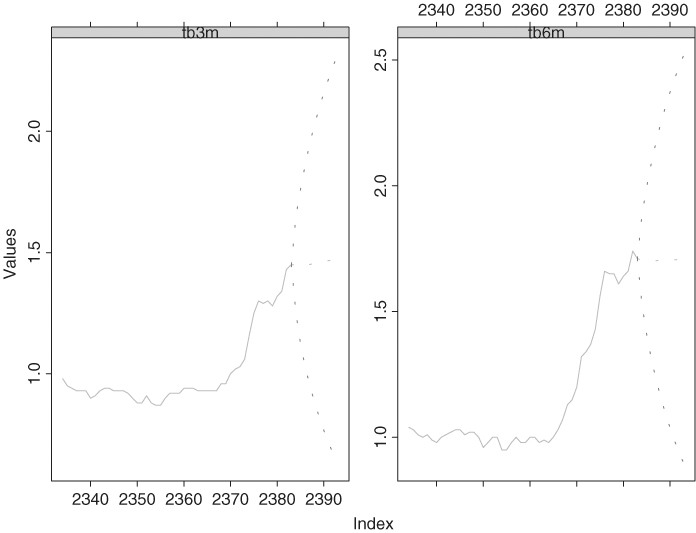
The forecasts are shown in Figures 8.14 and 8.15 for the differenced data and the original series, respectively, along with some observed data points. The dashed lines in the plots are pointwise 95% confidence intervals. Because of unit-root nonstationarity, the intervals are wide and not informative.
Figure 8.14 Forecasting plots of fitted ECM model for weekly U.S. interest rate series. Forecasts are for differenced series and forecast origin is August 6, 2004.

Figure 8.15 Forecasting plots of fitted ECM model for weekly U.S. interest rate series. Forecasts are for interest rates and forecast origin is August 6, 2004.
Remark
The package urca of R can be used to perform Johansen's co-integration test. The command is ca.jo. It requires specification of some subcommands. See the section of pairs trading for demonstration.