8.1 Weak Stationarity and Cross-Correlation Matrices

Consider a k-dimensional time series . The series is weakly stationary if its first and second moments are time invariant. In particular, the mean vector and covariance matrix of a weakly stationary series are constant over time. Unless stated explicitly to the contrary, we assume that the return series of financial assets are weakly stationary.

For a weakly stationary time series , we define its mean vector and covariance matrix as

8.1

where the expectation is taken element by element over the joint distribution of

. The mean is a k-dimensional vector consisting of the unconditional expectations of the components of . The covariance matrix is a k × k matrix. The ith diagonal element of is the variance of rit, whereas the (i, j)th element of is the covariance between rit and rjt. We write and when the elements are needed.

8.1.1 Cross-Correlation Matrices

Let be a k × k diagonal matrix consisting of the standard deviations of rit for i = 1, … , k. In other words, = diag. The concurrent, or lag-zero, cross-correlation matrix of is defined as

More specifically, the (i, j)th element of is

which is the correlation coefficient between rit and rjt. In time series analysis, such a correlation coefficient is referred to as a concurrent, or contemporaneous, correlation coefficient because it is the correlation of the two series at time t. It is easy to see that ρij(0) = ρji(0), − 1 ≤ ρij(0) ≤ 1, and ρii(0) = 1 for 1 ≤ i, j ≤ k. Thus, is a symmetric matrix with unit diagonal elements.

An important topic in multivariate time series analysis is the lead–lag relationships between component series. To this end, the cross-correlation matrices are used to measure the strength of linear dependence between time series. The lag-ℓ cross-covariance matrix of is defined as

8.2

where is the mean vector of . Therefore, the (i, j)th element of is the covariance between rit and rj, t−ℓ. For a weakly stationary series, the cross-covariance matrix is a function of ℓ, not the time index t.

The lag-ℓ cross-correlation matrix (CCM) of

is defined as

8.3

where, as before, is the diagonal matrix of standard deviations of the individual series rit. From the definition,

8.4

which is the correlation coefficient between rit and rj, t−ℓ. When ℓ > 0, this correlation coefficient measures the linear dependence of rit on rj, t−ℓ, which occurred prior to time t. Consequently, if ρij(ℓ) ≠ 0 and ℓ > 0, we say that the series rjt leads the series rit at lag ℓ. Similarly, ρji(ℓ) measures the linear dependence of rjt and ri, t−ℓ, and we say that the series rit leads the series rjt at lag ℓ if ρji(ℓ) ≠ 0 and ℓ > 0. Equation (8.4) also shows that the diagonal element ρii(ℓ) is simply the lag-ℓ autocorrelation coefficient of rit.

Based on this discussion, we obtain some important properties of the cross correlations when ℓ > 0. First, in general, ρij(ℓ) ≠ ρji(ℓ) for i ≠ j because the two correlation coefficients measure different linear relationships between {rit} and {rjt}. Therefore, and are in general not symmetric. Second, using Cov(x, y) = Cov(y, x) and the weak stationarity assumption, we have

so that Γij(ℓ) = Γji( − ℓ). Because Γji( − ℓ) is the (j, i)th element of the matrix and the equality holds for 1 ≤ i, j ≤ k, we have and = . Consequently, unlike the univariate case, for a general vector time series when ℓ > 0. Because = , it suffices in practice to consider the cross-correlation matrices for ℓ ≥ 0.

8.1.2 Linear Dependence

Considered jointly, the cross-correlation matrices of a weakly stationary vector time series contain the following information:

Therefore, if ρij(ℓ) = 0 for all ℓ > 0, then rit does not depend linearly on any past value rj, t−ℓ of the rjt series.

In general, the linear relationship between two time series {rit} and {rjt} can be summarized as follows:

The conditions stated earlier are sufficient conditions. A more informative approach to study the relationship between time series is to build a multivariate model for the series because a properly specified model considers simultaneously the serial and cross correlations among the series.

8.1.3 Sample Cross-Correlation Matrices

Given the data , the cross-covariance matrix can be estimated by

8.5

where is the vector of sample means. The cross-correlation matrix is estimated by

8.6

where is the k × k diagonal matrix of the sample standard deviations of the component series.

Similar to the univariate case, asymptotic properties of the sample cross-correlation matrix have been investigated under various assumptions; see, for instance, Fuller (1976, Chapter 6). The estimate is consistent but is biased in a finite sample. For asset return series, the finite sample distribution of is rather complicated partly because of the presence of conditional heteroscedasticity and high kurtosis. If the finite-sample distribution of cross correlations is needed, we recommend that proper bootstrap resampling methods be used to obtain an approximate estimate of the distribution. For many applications, a crude approximation of the variance of is sufficient.

Example 8.1

Consider the monthly log returns of IBM stock and the S&P 500 index from January 1926 to December 2008 with 996 observations. The returns include dividend payments and are in percentages. Denote the returns of IBM stock and the S&P 500 index by r1t and r2t, respectively. These two returns form a bivariate time series . Figure 8.1 shows the time plots of . Figure 8.2 shows some scatterplots of the two series. The plots show that the two return series are concurrently correlated. Indeed, the sample concurrent correlation coefficient between the two returns is 0.65, which is statistically significant at the 5% level. However, the cross correlations at lag 1 are weak if any.

Figure 8.1 Time plots of monthly log returns, in percentages, for (a) IBM stock and (b) the S&P 500 index from January 1926 to December 2008.

Figure 8.2 Some scatterplots for monthly log returns of IBM stock and S&P 500 index: (a) concurrent plot of IBM vs. S&P 500, (b) S&P 500 vs. lag-1 IBM, (c) IBM vs. lag-1 S&P 500, and (d) S&P 500 vs. lag-1 S&P 500.

Table 8.1 provides some summary statistics and cross-correlation matrices of the two series. For a bivariate series, each CCM is a 2 × 2 matrix with four correlations. Empirical experience indicates that it is rather hard to absorb simultaneously many cross-correlation matrices, especially when the dimension k is greater than 3. To overcome this difficulty, we use the simplifying notation of Tiao and Box (1981) and define a simplified cross-correlation matrix consisting of three symbols “ + ,” “−,” and “.” where they have the following meaning:

1. Plus sign ( + ) means that the corresponding correlation coefficient is greater than or equal to .

2. Minus sign (−) means that the corresponding correlation coefficient is less than or equal to .

3. Period (.) means that the corresponding correlation coefficient is between and .

And is the asymptotic 5% critical value of the sample correlation under the assumption that is a white noise series.

Table 8.1 Summary Statistics and Cross-Correlation Matrices of Monthly Log Returns of IBM Stock and S&P 500 Index: January 1926 to December 2008

Table 8.1(c) shows the simplified CCM for the monthly log returns of IBM stock and the S&P 500 index. It is easily seen that significant cross correlations at the approximate 5% level appear mainly at lags 1 and 3. An examination of the sample CCMs at these two lags indicates that (a) S&P 500 index returns have some marginal autocorrelations at lags 1, 2, 3, and 5 and (b) IBM stock returns depend weakly on the previous returns of the S&P 500 index. The latter observation is based on the significance of cross correlations at the (1, 2)th element of lag-1, lag-2 and lag-5 CCMs.

Figure 8.3 shows the sample autocorrelations and cross correlations of the two series. The upper-left plot is the sample ACF of IBM stock returns and the upper-right plot shows the dependence of IBM stock returns on the lagged S&P 500 index returns. The dashed lines in the plots are the asymptotic two standard error limits of the sample auto- and cross-correlation coefficients. From the plots, the dynamic relationship is weak between the two return series, but their contemporaneous correlation is statistically significant.

Figure 8.3 Sample auto- and cross-correlation functions (CCF) of two monthly log return series: (a) sample ACF of IBM stock returns, (b) cross-correlations between S&P 500 index and lagged IBM stock returns (lower left), (c) cross correlations between IBM stock and lagged S&P 500 index returns, and (d) sample ACF of S&P 500 index returns. Dashed lines denote 95% limits.

Example 8.2

Consider the simple returns of monthly indexes of U.S. government bonds with maturities in 30 years, 20 years, 10 years, 5 years, and 1 year. The data obtained from the CRSP database have 696 observations starting from January 1942 to December 1999. Let be the return series with decreasing time to maturity. Figure 8.4 shows the time plots of on the same scale. The variability of the 1-year bond returns is much smaller than that of returns with longer maturities. The sample means and standard deviations of the data are and . The concurrent correlation matrix of the series is

It is not surprising that (a) the series have high concurrent correlations, and (b) the correlations between long-term bonds are higher than those between short-term bonds.

Figure 8.4 Time plots of monthly simple returns of five indexes of U.S. government bonds with maturities in (a) 30 years, (b) 20 years, (c) 10 years, (d) 5 years, and (e) 1 year. Sample period is from January 1942 to December 1999.

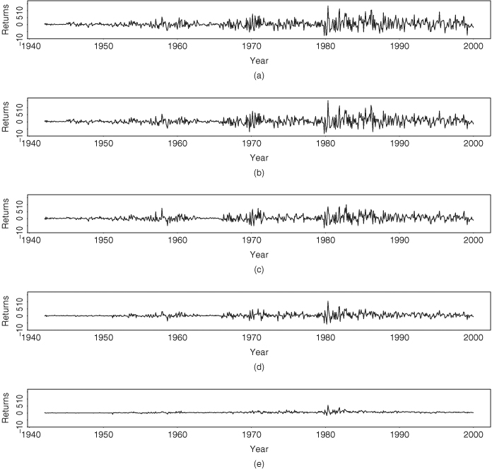
Table 8.2 gives the lag-1 and lag-2 cross-correlation matrices of and the corresponding simplified matrices. Most of the significant cross correlations are at lag 1, and the five return series appear to be intercorrelated. In addition, lag-1 and lag-2 sample ACFs of the 1-year bond returns are substantially higher than those of other series with longer maturities.

Table 8.2 Sample Cross-Correlation Matrices of Monthly Simple Returns of Five Indexes of U.S. Government Bonds: January 1942 to December 1999

8.1.4 Multivariate Portmanteau Tests

The univariate Ljung–Box statistic Q(m) has been generalized to the multivariate case by Hosking (1980, 1981) and Li and McLeod (1981). For a multivariate series, the null hypothesis of the test statistic is , and the alternative hypothesis for some i ∈ {1, … , m}. Thus, the statistic is used to test that there are no auto- and cross correlations in the vector series . The test statistic assumes the form

8.7

where T is the sample size, k is the dimension of , and is the trace of the matrix , which is the sum of the diagonal elements of . Under the null hypothesis and some regularity conditions, Qk(m) follows asymptotically a chi-squared distribution with k2m degrees of freedom.

Applying the Qk(m) statistics to the bivariate monthly log returns of IBM stock and the S&P 500 index of Example 8.1, we have Q2(1) = 9.81, Q2(5) = 47.06, and Q2(10) = 71.65. Based on asymptotic chi-squared distributions with degrees of freedom 4, 20, and 40, the p values of these Q2(m) statistics are 0.044, 0.001, and 0.002, respectively. The portmanteau tests thus confirm the existence of serial dependence in the bivariate return series at the 5% significance level. For the five-dimensional monthly simple returns of bond indexes in Example 8.2, we have Q5(5) = 1065.63, which is highly significant compared with a chi-squared distribution with 125 degrees of freedom.

The Qk(m) statistic is a joint test for checking the first m cross-correlation matrices of being zero. If it rejects the null hypothesis, then we build a multivariate model for the series to study the lead–lag relationships between the component series. In what follows, we discuss some simple vector models useful for modeling the linear dynamic structure of a multivariate financial time series.