12.7 Stochastic Volatility Models
An important financial application of MCMC methods is the estimation of stochastic volatility models; see Jacquier, Polson, and Rossi (1994) and the references therein. We start with a univariate stochastic volatility model. The mean and volatility equations of an asset return rt are
where {xit|i = 1, … , p} are explanatory variables available at time t − 1, the βj are parameters, {ϵt} is a Gaussian white noise sequence with mean 0 and variance 1, {vt} is also a Gaussian white noise sequence with mean 0 and variance ![]() , and {ϵt} and {vt} are independent. The log transformation is used to ensure that ht is positive for all t. The explanatory variables xit may include lagged values of the return (e.g., xit = rt−i). In Eq. (12.21), we assume that |α1| < 1 so that the log volatility process ln ht is stationary. If necessary, a higher order AR(p) model can be used for ln ht.
, and {ϵt} and {vt} are independent. The log transformation is used to ensure that ht is positive for all t. The explanatory variables xit may include lagged values of the return (e.g., xit = rt−i). In Eq. (12.21), we assume that |α1| < 1 so that the log volatility process ln ht is stationary. If necessary, a higher order AR(p) model can be used for ln ht.
Denote the coefficient vector of the mean equation by ![]() = (β0, β1, … , βp)′ and the parameter vector of the volatility equation by
= (β0, β1, … , βp)′ and the parameter vector of the volatility equation by ![]() . Suppose that
. Suppose that ![]() is the collection of observed returns and
is the collection of observed returns and ![]() is the collection of explanatory variables. Let
is the collection of explanatory variables. Let ![]() be the vector of unobservable volatilities. Here
be the vector of unobservable volatilities. Here ![]() and
and ![]() are the “traditional” parameters of the model and
are the “traditional” parameters of the model and ![]() is an auxiliary variable. Estimation of the model would be complicated via the maximum-likelihood method because the likelihood function is a mixture over the n-dimensional
is an auxiliary variable. Estimation of the model would be complicated via the maximum-likelihood method because the likelihood function is a mixture over the n-dimensional ![]() distribution as
distribution as
![]()
However, under the Bayesian framework, the volatility vector ![]() consists of augmented parameters. Conditioning on
consists of augmented parameters. Conditioning on ![]() , we can focus on the probability distribution functions
, we can focus on the probability distribution functions ![]() and
and ![]() and the prior distribution
and the prior distribution ![]() . We assume that the prior distribution can be partitioned as
. We assume that the prior distribution can be partitioned as ![]() ; that is, prior distributions for the mean and volatility equations are independent. A Gibbs sampling approach to estimating the stochastic volatility in Eqs. (12.20) and (12.21) then involves drawing random samples from the following conditional posterior distributions:
; that is, prior distributions for the mean and volatility equations are independent. A Gibbs sampling approach to estimating the stochastic volatility in Eqs. (12.20) and (12.21) then involves drawing random samples from the following conditional posterior distributions:
![]()
In what follows, we give details of practical implementation of the Gibbs sampling used.
12.7.1 Estimation of Univariate Models
Given ![]() , the mean equation in (12.20) is a nonhomogeneous linear regression. Dividing the equation by
, the mean equation in (12.20) is a nonhomogeneous linear regression. Dividing the equation by ![]() , we can write the model as
, we can write the model as
where ![]() and
and ![]() , with
, with ![]() being the vector of explanatory variables. Suppose that the prior distribution of
being the vector of explanatory variables. Suppose that the prior distribution of ![]() is multivariate normal with mean
is multivariate normal with mean ![]() and covariance matrix
and covariance matrix ![]() . Then the posterior distribution of
. Then the posterior distribution of ![]() is also multivariate normal with mean
is also multivariate normal with mean ![]() and covariance matrix
and covariance matrix ![]() . These two quantities can be obtained as before via Result 12.1a, and they are
. These two quantities can be obtained as before via Result 12.1a, and they are
![]()
where it is understood that the summation starts with p + 1 if rt−p is the highest lagged return used in the explanatory variables.
The volatility vector ![]() is drawn element by element. The necessary conditional posterior distribution is
is drawn element by element. The necessary conditional posterior distribution is ![]() , which is produced by the normal distribution of at and the lognormal distribution of the volatility,
, which is produced by the normal distribution of at and the lognormal distribution of the volatility,
where ![]() and
and ![]() . Here we have used the following properties: (a) at|ht ∼ N(0, ht); (b)
. Here we have used the following properties: (a) at|ht ∼ N(0, ht); (b) ![]() ; (c)
; (c) ![]() ; (d)
; (d) ![]() , where d denotes differentiation; and (e) the equality
, where d denotes differentiation; and (e) the equality
![]()
where c = (Aa + Cb)/(A + C) provided that A + C ≠ 0. This equality is a scalar version of Lemma 1 of Box and Tiao (1973, p. 418). In our application, A = 1, a = α0 + ln ht−1, ![]() , and b = (ln ht+1 − α0)/α1. The term (a − b)2AC/(A + C) does not contain the random variable ht and, hence, is integrated out in the derivation of the conditional posterior distribution. Jacquier, Polson, and Rossi (1994) use the Metropolis algorithm to draw ht. We use Griddy Gibbs in this section, and the range of ht is chosen to be a multiple of the unconditional sample variance of rt.
, and b = (ln ht+1 − α0)/α1. The term (a − b)2AC/(A + C) does not contain the random variable ht and, hence, is integrated out in the derivation of the conditional posterior distribution. Jacquier, Polson, and Rossi (1994) use the Metropolis algorithm to draw ht. We use Griddy Gibbs in this section, and the range of ht is chosen to be a multiple of the unconditional sample variance of rt.
To draw random samples of ![]() , we partition the parameters as
, we partition the parameters as ![]() and
and ![]() . The prior distribution of
. The prior distribution of ![]() is also partitioned accordingly [i.e.,
is also partitioned accordingly [i.e., ![]() ]. The conditional posterior distributions needed are
]. The conditional posterior distributions needed are
 : Given
  , ln ht follows an AR(1) model. Therefore, the result of AR models discussed in the previous two sections applies. Specifically, if the prior distribution of
  is multivariate normal with mean
  and covariance matrix Co, then
  is multivariate normal with mean
  and covariance matrix
  , where
![]()
where ![]() .
.
 : Given
  and
and  , we can calculate vt = ln ht − α0 − α1 ln ht−1 for t = 2, … , n. Therefore, if the prior distribution of
  is
is  , then the conditional posterior distribution of
  is an inverted chi-squared distribution with m + n − 1 degrees of freedom; that is,
![]()
Remark
Formula (12.23) is for 1 < t < n, where n is the sample size. For the two end data points h1 and hn, some modifications are needed. A simple approach is to assume that h1 is fixed so that the drawing of ht starts with t = 2. For t = n, one uses the result ![]() . Alternatively, one can employ a forecast of hn+1 and a backward prediction of h0 and continue to apply the formula. Since hn is the variable of interest, we forecast hn+1 by using a 2-step-ahead forecast at the forecast origin n − 1. For the model in Eq. (12.21), the forecast of hn+1 is
. Alternatively, one can employ a forecast of hn+1 and a backward prediction of h0 and continue to apply the formula. Since hn is the variable of interest, we forecast hn+1 by using a 2-step-ahead forecast at the forecast origin n − 1. For the model in Eq. (12.21), the forecast of hn+1 is
![]()
The backward prediction of h0 is based on the time reversibility of the model
![]()
where η = α0/(1 − α1) and |α1| < 1. The model of the reversed series is
![]()
where η = α0/(1 - α1) is also a Gaussian white noise series with mean zero and variance ![]() . Consequently, the 2-step-backward prediction of h0 at time t = 2 is
. Consequently, the 2-step-backward prediction of h0 at time t = 2 is
![]() □
□
Remark
Formula (12.23) can also be obtained by using results of a missing value in an AR(1) model; see Section 12.6.1. Specifically, assume that ln ht is missing. For the AR(1) model in Eq. (12.21), this missing value is related to ln ht−1 and ln ht+1 for 1 < t < n. From the model, we have
![]()
Define yt = α0 + α1yt−1, xt = 1, and bt = − at. Then we obtain
Next, from
![]()
we define yt+1 = ln ht+1 − α0, xt+1 = α1, and bt+1 = at+1 and obtain
Now Eqs. (12.24) and (12.25) form a special simple linear regression with two observations and an unknown parameter ln ht. Note that bt and bt+1 have the same distribution because − at is also ![]() . The least-squares estimate of ln ht is then
. The least-squares estimate of ln ht is then
![]()
which is precisely the conditional mean of ln ht given in Eq. (12.23). In addition, this estimate is normally distributed with mean ln ht and variance ![]() . Formula (12.23) is simply the product of at ∼ N(0, ht) and
. Formula (12.23) is simply the product of at ∼ N(0, ht) and ![]() with the transformation
with the transformation ![]() . This regression approach generalizes easily to other AR(p) models for ln ht. We use this approach and assume that
. This regression approach generalizes easily to other AR(p) models for ln ht. We use this approach and assume that ![]() are fixed for a stochastic volatility AR(p) model. □
are fixed for a stochastic volatility AR(p) model. □
Remark
Starting value of ht can be obtained by fitting a volatility model of Chapter 3 to the return series. □
Example 12.3
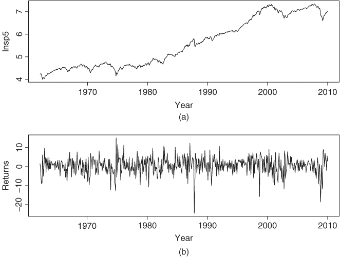
Consider the monthly log returns of the S&P 500 index from January 1962 to December 2009 for 575 observations. The returns are computed using the first adjusted closing index of each month, that is, the closing index of the first trading day of each month. Figure 12.4(a) shows the time plot of the log level of the index, whereas Figure 12.4(b) shows the log returns measured in percentage. If GARCH models are entertained for the series, we obtain a Gaussian GARCH(1,1) model
where t ratios of the coefficients are all greater than 2.56. The Ljung–Box statistics of the standardized residuals and their squared series fail to indicate any model inadequacy. Specifically, we have Q(12) = 10.04(0.61) and 6.14(0.91), respectively, for the standardized residuals and their squared series.
Figure 12.4 Time plot of monthly S&P 500 index from 1962 to 2009: (a) log level and (b) log return in percentage.
Next, consider the stochastic volatility model
where the vt are iid ![]() . To implement the Gibbs sampling, we use the prior distributions
. To implement the Gibbs sampling, we use the prior distributions
![]()
where ![]() . For initial parameter values, we use the fitted values of the GARCH(1,1) model in Eq. (12.26) for {ht}, that is, h0t = ht, and set
. For initial parameter values, we use the fitted values of the GARCH(1,1) model in Eq. (12.26) for {ht}, that is, h0t = ht, and set ![]() and
and ![]() to the least-squares estimate of ln(h0t). The initial value of μ is the sample mean of the log returns. The volatility ht is drawn by the Griddy Gibbs with 400 grid points. The possible range of ht for the jth Gibbs iteration is [η1t, η2t], where η1t = 0.6 × max(hj−1, t, h0t) and η2t = 1.4 × min(hj−1, t, h0t), where hj−1, t and h0t denote, respectively, the estimate of ht for the (j − 1)th iteration and initial value.
to the least-squares estimate of ln(h0t). The initial value of μ is the sample mean of the log returns. The volatility ht is drawn by the Griddy Gibbs with 400 grid points. The possible range of ht for the jth Gibbs iteration is [η1t, η2t], where η1t = 0.6 × max(hj−1, t, h0t) and η2t = 1.4 × min(hj−1, t, h0t), where hj−1, t and h0t denote, respectively, the estimate of ht for the (j − 1)th iteration and initial value.
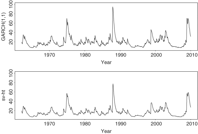
We ran the Gibbs sampling for 2500 iterations but discarded results of the first 500 iterations. Figure 12.5 shows the density functions of the prior and posterior distributions of the four coefficient parameters. The prior distributions used are relatively noninformative. The posterior distributions are concentrated especially for μ and ![]() . Figure 12.6 shows the time plots of fitted volatilities. The upper panel shows the posterior mean of ht over the 5000 iterations for each time point, whereas the lower panel shows the fitted values of the GARCH(1,1) model in Eq. (12.26). The two plots exhibit a similar pattern.
. Figure 12.6 shows the time plots of fitted volatilities. The upper panel shows the posterior mean of ht over the 5000 iterations for each time point, whereas the lower panel shows the fitted values of the GARCH(1,1) model in Eq. (12.26). The two plots exhibit a similar pattern.
Figure 12.5 Density functions of prior and posterior distributions of parameters in stochastic volatility model for monthly log returns of S&P 500 index. Dashed line denotes prior density and solid line the posterior density, which is based on results of Gibbs sampling with 2000 iterations. See text for more details.
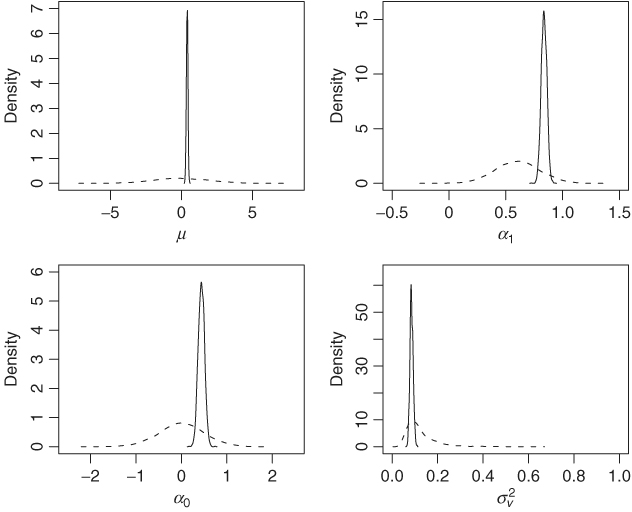
Figure 12.6 Time plots of fitted volatilities for monthly log returns of S&P 500 index from 1962 to 2009. Lower panel shows posterior means of a Gibbs sampler with 2000 iterations. Upper panel shows results of a Gaussian GARCH(1,1) model.
The posterior mean and standard error of the four coefficients are as follows:
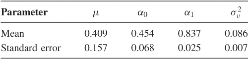
The posterior mean of α1 is 0.837, confirming strong serial dependence in the volatility series. This value is smaller than that obtained by Jacquier, Polson, and Rossi (1994) who used daily returns of the S&P 500 index. Finally, we have used different initial values, priors, and numbers of iterations for the Gibbs sampler. The results are stable. Of course, as expected, the results and efficiency of the Griddy Gibbs algorithm depend on the specification of the range for ht.
12.7.2 Multivariate Stochastic Volatility Models
In this section, we study multivariate stochastic volatility models using the Cholesky decomposition of Chapter 10. We focus on the bivariate case, but the methods discussed also apply to the higher dimensional case. Based on the Cholesky decomposition, the innovation ![]() of a return series
of a return series ![]() is transformed into
is transformed into ![]() such that
such that
![]()
where b2t and q21, t can be interpreted as the residual and least-squares estimate of the linear regression
![]()
The conditional covariance matrix of ![]() is parameterized by {g11, t, g22, t} and {q21, t} as
is parameterized by {g11, t, g22, t} and {q21, t} as
where gii, t = Var(bit|Ft−1) and b1t⊥b2t. Thus, the quantities of interest are g11, t, g22, t and q21, t.
A simple bivariate stochastic volatility model for the return ![]() is as follows:
is as follows:
where ![]() is a sequence of serially uncorrelated Gaussian random vectors with mean zero and conditional covariance matrix
is a sequence of serially uncorrelated Gaussian random vectors with mean zero and conditional covariance matrix ![]() given by Eq. (12.28),
given by Eq. (12.28), ![]() is a two-dimensional constant vector,
is a two-dimensional constant vector, ![]() denotes the explanatory variables, and {v1t}, {v2t}, and {ut} are three independent Gaussian white noise series such that Var(vit) =
denotes the explanatory variables, and {v1t}, {v2t}, and {ut} are three independent Gaussian white noise series such that Var(vit) = ![]() and Var(ut) =
and Var(ut) = ![]() . Again log transformation is used in Eq. (12.30) to ensure the positiveness of gii, t.
. Again log transformation is used in Eq. (12.30) to ensure the positiveness of gii, t.
Let ![]() ,
, ![]() , and
, and ![]() . The “traditional” parameters of the model in Eqs. (12.29)–(12.31) are
. The “traditional” parameters of the model in Eqs. (12.29)–(12.31) are ![]() ,
, ![]() , and
, and ![]() for i = 1, 2, and
for i = 1, 2, and ![]() and
and ![]() . The augmented parameters are
. The augmented parameters are ![]() ,
, ![]() , and
, and ![]() . To estimate such a bivariate stochastic volatility model via Gibbs sampling, we use results of the univariate model in the previous section and two additional conditional posterior distributions. Specifically, we can draw random samples of
. To estimate such a bivariate stochastic volatility model via Gibbs sampling, we use results of the univariate model in the previous section and two additional conditional posterior distributions. Specifically, we can draw random samples of
1. ![]() and
and ![]() row by row using the result (12.22)
row by row using the result (12.22)
2. g11, t using Eq. (12.23) with at being replaced by a1t
3. ![]() and
and ![]() using exactly the same methods as those of the univariate case with at replaced by a1t
using exactly the same methods as those of the univariate case with at replaced by a1t
To draw random samples of ![]() ,
, ![]() , and g22, t, we need to compute b2t. But this is easy because b2t = a2t − q21, ta1t given the augmented parameter vector
, and g22, t, we need to compute b2t. But this is easy because b2t = a2t − q21, ta1t given the augmented parameter vector ![]() . Furthermore, b2t is normally distributed with mean 0 and conditional variance g22, t.
. Furthermore, b2t is normally distributed with mean 0 and conditional variance g22, t.
It remains to consider the conditional posterior distributions
![]()
where ![]() denotes the collection of
denotes the collection of ![]() , which is known if
, which is known if ![]() ,
, ![]() ,
, ![]() , and
, and ![]() are given. Given
are given. Given ![]() and
and ![]() , model (12.31) is a simple Gaussian AR(1) model. Therefore, if the prior distribution of
, model (12.31) is a simple Gaussian AR(1) model. Therefore, if the prior distribution of ![]() is bivariate normal with mean
is bivariate normal with mean ![]() and covariance matrix
and covariance matrix ![]() , then the conditional posterior distribution of
, then the conditional posterior distribution of ![]() is also bivariate normal with mean
is also bivariate normal with mean ![]() and covariance matrix
and covariance matrix ![]() , where
, where
![]()
where ![]() . Similarly, if the prior distribution of
. Similarly, if the prior distribution of  is
is ![]() , then the conditional posterior distribution of
, then the conditional posterior distribution of ![]() is
is
![]()
where ut = q21, t − γ0 − γ1q21, t−1. Finally,
where ![]() and
and ![]() . In general, μt and σ2 can be obtained by using the results of a missing value in an AR(p) process. It turns out that Eq. (12.32) has a closed-form distribution for q21, t. Specifically, the first term of Eq. (12.32), which is the conditional distribution of q21, t given g22, t and
. In general, μt and σ2 can be obtained by using the results of a missing value in an AR(p) process. It turns out that Eq. (12.32) has a closed-form distribution for q21, t. Specifically, the first term of Eq. (12.32), which is the conditional distribution of q21, t given g22, t and ![]() , is normal with mean a2t/a1t and variance g22, t/(a1t)2. The second term of the equation is also normal with mean μt and variance σ2. Consequently, by Result 12.1, the conditional posterior distribution of q21, t is normal with mean μ* and variance
, is normal with mean a2t/a1t and variance g22, t/(a1t)2. The second term of the equation is also normal with mean μt and variance σ2. Consequently, by Result 12.1, the conditional posterior distribution of q21, t is normal with mean μ* and variance ![]() , where
, where
![]()
where μt is defined in Eq. 12.32.
Example 12.4
In this example, we study bivariate volatility models for the monthly log returns of IBM stock and the S&P 500 index from January 1962 to December 2009. This is an expanded version of Example 12.3 by adding the IBM returns. Figure 12.7 shows the time plots of the two return series. Let ![]() = (IBMt, SPt)′. If time-varying correlation GARCH models with Cholesky decomposition of Chapter 10 are entertained, we obtain the model
= (IBMt, SPt)′. If time-varying correlation GARCH models with Cholesky decomposition of Chapter 10 are entertained, we obtain the model
12.35 ![]()
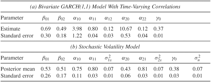
where b2t = a2t − q21, ta1t and the estimates and their standard errors are given in Table 12.2(a). For comparison purpose, we also fit a BEKK(1,1) model and obtain ![]() and the coefficient matrices
and the coefficient matrices
![]()
where the matrices are defined in Eq. (10.6) of Chapter 10.
Figure 12.7 Time plots of monthly log returns of (a) IBM stock and (b) S&P 500 index from 1962 to 2009.
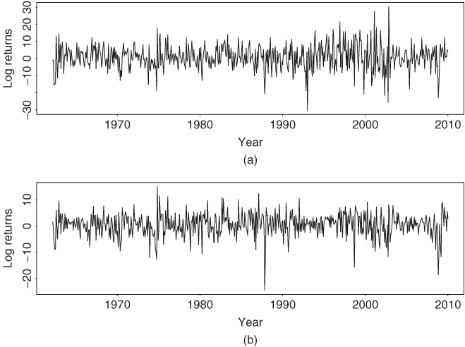
Table 12.2 Estimation of Bivariate Volatility Models for Monthly Log Returns of IBM Stock and S&P 500 Index from January 1962 to December 2009a
a
The stochastic volatility models are based on the last 2000 iterations of a Gibbs sampling with 2500 total iterations.
For stochastic volatility model, we employ the same mean equation in Eq. (12.33) and a stochastic volatility model similar to that in Eqs. (12.34)–(12.36). The volatility equations are
12.37 ![]()
12.38 ![]()
12.39 ![]()
The prior distributions used are
where i = 1 and 2. These prior distributions are relatively noninformative. We obtained the initial values of {g11, t, g22, t, q21, t} from the results of the BEKK(1,1) model. In addition, we set the values of quantities at t = 1 as given. We then ran the Gibbs sampling for 2500 iterations but discarded results of the first 500 iterations. The random samples of gii, t were drawn by Griddy Gibbs with 500 grid points in the intervals [ηi, 1t, ηi, 2t] where the lower and upper bounds are set by the same method as those of Example 12.3. Posterior means and standard errors of the “traditional” parameters of the bivariate stochastic volatility model are given in Table 12.2(b).
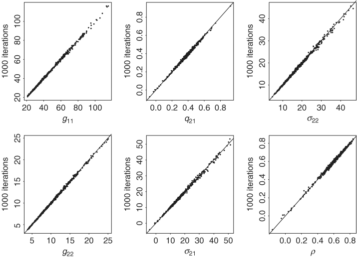
To check for convergence of the Gibbs sampling, we ran the procedure several times with different starting values and numbers of iterations. The results are stable. For illustration, Figure 12.8 shows the scatterplots of various quantities for two different Gibbs samples. The first Gibbs sample is based on 500 + 2000 iterations, and the second Gibbs sample is based on 500 + 1000 iterations, where M + N denotes that the total number of Gibbs iterations is M + N, but results of the first M iterations are discarded. The scatterplots shown are posterior means of g11, t, g22, t, g21, t, σ22, t, σ21, t, and the correlation ρ21, t. The line y = x is added to each plot to show the closeness of the posterior means. The stability of the Gibbs sampling results is clearly seen.
Figure 12.8 Scatterplots of posterior means of various statistics of two different Gibbs samples for bivariate stochastic volatility model for monthly log returns of IBM stock and S&P 500 index. The x axis denotes results based on 500 + 2000 iterations and the y axis denotes results based on 500 + 1000 iterations. Notation is defined in text.
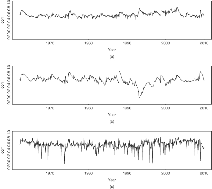
It is informative to compare the BEKK model and the GARCH model with time-varying correlations in Eqs. (12.33)–(12.36) with the stochastic volatility model. First, as expected, the mean equations of the three models are essentially identical. Second, Figure 12.9 shows the time plots of the conditional variance for IBM stock return. Figure 12.9(a) is for the GARCH model, Figure 12.9(b) is from the BEKK model, and Figure 12.9(c) shows the posterior mean of the stochastic volatility model. The three models show similar volatility characteristics; they exhibit volatility clustering and indicate an increasing trend in volatility. However, the GARCH model produces higher peak volatility values and an additional peak in 1993. Third, Figure 12.10 shows the time plots of conditional variance for the S&P 500 index return. The GARCH model produces an extra volatility peak around 1993. This additional peak does not appear in the univariate analysis shown in Figure 12.6. It seems that for this particular instance the bivariate GARCH model produces a spurious volatility peak. This spurious peak is induced by its dependence on IBM returns and does not appear in the stochastic volatility model or the BEKK model. Indeed, the fitted volatilities of the S&P 500 index return by the bivariate stochastic volatility model are similar to that of the univariate analysis. Fourth, Figure 12.11 shows the time plots of fitted conditional correlations. Here the three models differ substantially. The correlations of the GARCH model with Cholesky decomposition are relatively smooth and always positive with mean value 0.59 and standard deviation 0.07. The range of the correlations is (0.411,0.849). The correlations of the BEKK(1,1) model assume small negative values around 1993 and are more variable with mean 0.59, standard deviation 0.13 and range (− 0.020, 0.877). However, the correlations produced by the stochastic volatility model vary markedly from one month to another with mean value 0.60, standard deviation 0.14, and range (− 0.161, 0.839). Furthermore, the negative correlations occur in several isolated periods. The difference is understandable because q21, t contains the random shock ut in the stochastic volatility model.
Remark
The Gibbs sampling estimation applies to other bivariate stochastic volatility models. The conditional posterior distributions needed require some extensions of those discussed in this section, but they are based on the same ideas. The BEKK model is estimated by using Matlab. □
Figure 12.9 Time plots of fitted conditional variance for monthly log returns of IBM stock from 1962 to 2009: (a) GARCH model with time-varying correlations, (b) BEKK(1,1) model, and (c) bivariate stochastic volatility model estimated by Gibbs sampling with 500 + 2000 iterations.
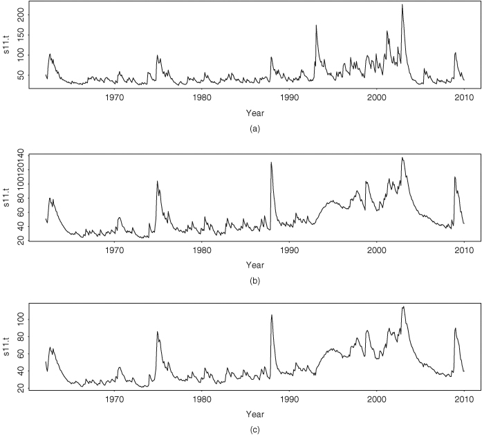
Figure 12.10 Time plots of conditional variance for monthly log returns of S&P 500 index from 1962 to 2009: (a) GARCH model with time-varying correlations, (b) BEKK(1,1) model, and (c) bivariate stochastic volatility model estimated by Gibbs sampling with 500 + 2000 iterations.
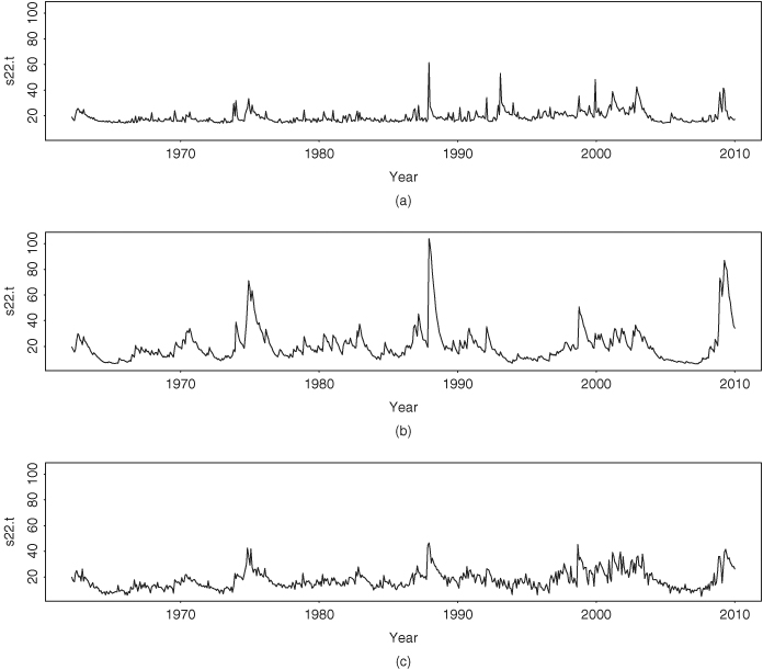
Figure 12.11 Time plots of fitted correlation coefficients between monthly log returns of IBM stock and S&P 500 index from 1962 to 2009: (a) GARCH model with time-varying correlations, (b) BEKK(1,1) model, and (c) bivariate stochastic volatility model estimated by Gibbs sampling with 500 + 2000 iterations.