
12.8 New Approach to SV Estimation
In this section, we discuss an alternative procedure to estimate stochastic volatility (SV) models. This approach makes use of the technique of forward filtering and backward sampling (FFBS) within the Kalman filter framework to improve the efficiency of Gibbs sampling. It can dramatically reduce the computing time by drawing the volatility process jointly with the help of a mixture of normal distributions. In fact, the approach can be used to estimate many stochastic diffusion models with leverage effects and jumps.
For ease in presentation, we reparameterize the univariate stochastic volatility model in Eqs. (12.20) and (12.21) as
where ![]() ,
, ![]() , σ0 > 0, {zt} is a zero-mean log volatility series, and {ϵt} and {ηt} are bivariate normal distributions with mean zero and covariance matrix
, σ0 > 0, {zt} is a zero-mean log volatility series, and {ϵt} and {ηt} are bivariate normal distributions with mean zero and covariance matrix
![]()
The parameter ρ is the correlation between ϵt and ηt and represents the leverage effect of the asset return rt. Typically, ρ is negative signifying that a negative return tends to increase the volatility of an asset price.
Compared with the model in Eqs. (12.22) and (12.20), we have ![]() and
and ![]() . That is, zt is a mean-adjusted log volatility series. This new parameterization has some nice characteristics. For example, the volatility series is σ0 exp(zt/2), which is always positive. More importantly, ηt is the innovation of zt+1 and is independent of zt. This simple time shift enables us to handle the leverage effect. If one postulates zt = αzt−1 + ηt for Eq. (12.41), then ηt and ϵt cannot be correlated because a nonzero correlation implies that zt and ϵt are correlated in Eq. (12.40), which would lead to some identifiability issues.
. That is, zt is a mean-adjusted log volatility series. This new parameterization has some nice characteristics. For example, the volatility series is σ0 exp(zt/2), which is always positive. More importantly, ηt is the innovation of zt+1 and is independent of zt. This simple time shift enables us to handle the leverage effect. If one postulates zt = αzt−1 + ηt for Eq. (12.41), then ηt and ϵt cannot be correlated because a nonzero correlation implies that zt and ϵt are correlated in Eq. (12.40), which would lead to some identifiability issues.
Remark
Alternatively, one can write the stochastic volatility model as
![]()
where (ϵt, ηt)′ is a bivariate normal distribution as before. Yet another equivalent parameterization is

where ![]() is not zero. □
is not zero. □
Parameters of the stochastic volatility model in Eqs. (12.40) and (12.41) are ![]() , and
, and ![]() , where n is the sample size. For simplicity, we assume z1 is known. To estimate these parameters via MCMC methods, we need their conditional posterior distributions. In what follows, we discuss the needed conditional posterior distributions.
, where n is the sample size. For simplicity, we assume z1 is known. To estimate these parameters via MCMC methods, we need their conditional posterior distributions. In what follows, we discuss the needed conditional posterior distributions.
1. Given ![]() and σ0 and a normal prior distribution,
and σ0 and a normal prior distribution, ![]() has the same conditional posterior distribution as that in Section 12.7.1 with
has the same conditional posterior distribution as that in Section 12.7.1 with ![]() replaced by σ0 exp(zt/2); see Eq. (12.22).
replaced by σ0 exp(zt/2); see Eq. (12.22).
2. Given ![]() and
and ![]() , α is a simple AR(1) coefficient. Thus, with an approximate normal prior, the conditional posterior distribution of α is readily available; see Section 12.7.1.
, α is a simple AR(1) coefficient. Thus, with an approximate normal prior, the conditional posterior distribution of α is readily available; see Section 12.7.1.
3. Given ![]() and
and ![]() , we define vt =
, we define vt = ![]() = σ0ϵt. Thus, {vt} is a sequence of iid normal random variables with mean zero and variance
= σ0ϵt. Thus, {vt} is a sequence of iid normal random variables with mean zero and variance ![]() . If the prior distribution of
. If the prior distribution of ![]() is
is ![]() , then the conditional posterior distribution of
, then the conditional posterior distribution of ![]() is an inverted chi-squared distribution with m + n degrees of freedom; that is,
is an inverted chi-squared distribution with m + n degrees of freedom; that is,
![]()
4. Given ![]() , σ0,
, σ0, ![]() , and α, we can easily obtain the bivariate innovation
, and α, we can easily obtain the bivariate innovation ![]() for t = 2, … , n. The likelihood function of
for t = 2, … , n. The likelihood function of ![]() is readily available as
is readily available as

where ![]() denotes trace of the matrix
denotes trace of the matrix ![]() . However, this joint distribution is complicated because one cannot separate ρ and
. However, this joint distribution is complicated because one cannot separate ρ and ![]() . We adopt the technique of Jacquier, Polson, and Rossi (2004) and reparameterize the covariance matrix as
. We adopt the technique of Jacquier, Polson, and Rossi (2004) and reparameterize the covariance matrix as
![]()
where ![]() . It is easy to see that
. It is easy to see that ![]() and
and
![]()
where ![]() contains φ only. Let
contains φ only. Let ![]() and
and ![]() be the innovations of the model in Eqs. (12.40) and (12.41). The likelihood function then becomes (keeping terms related to parameters only)
be the innovations of the model in Eqs. (12.40) and (12.41). The likelihood function then becomes (keeping terms related to parameters only)
![]()
where ![]() , which is the 2 × 2 cross-product matrix of the innovations. For simplicity, we use conjugate priors such that ω is inverse gamma (IG) with hyperparameters (γ0/2, γ1/2); that is, ω ∼ IG(γ0/2, γ1/2), and φ|ω ∼ N(0, ω/2). Then, after some algebraic manipulation, the joint posterior distribution of (φ, ω) can be decomposed into a normal and an inverse gamma distribution. Specifically,
, which is the 2 × 2 cross-product matrix of the innovations. For simplicity, we use conjugate priors such that ω is inverse gamma (IG) with hyperparameters (γ0/2, γ1/2); that is, ω ∼ IG(γ0/2, γ1/2), and φ|ω ∼ N(0, ω/2). Then, after some algebraic manipulation, the joint posterior distribution of (φ, ω) can be decomposed into a normal and an inverse gamma distribution. Specifically,
![]()
where ![]() , and
, and
![]()
In Gibbs sampling, once φ and ω are available, we can obtain ρ and ![]() easily because
easily because ![]() and ρ = φ/ση. Note that the probability density function of an IG(α, β) random variable ω is
and ρ = φ/ση. Note that the probability density function of an IG(α, β) random variable ω is
![]()
where α > 2 and β > 0.
5. Finally, we consider the joint distribution of the log volatility ![]() given the data and other parameters. From Eq. (12.40), we have
given the data and other parameters. From Eq. (12.40), we have
![]()
Therefore, letting ![]() , we obtain
, we obtain
where ![]() . Since
. Since ![]() ,
, ![]() is not normally distributed. Treating Eq. (12.42) as an observation equation and Eq. (12.40) as the state equation, we have the form of a state-space model except that
is not normally distributed. Treating Eq. (12.42) as an observation equation and Eq. (12.40) as the state equation, we have the form of a state-space model except that ![]() is not Gaussian; see Eqs. 11.26 and 11.27. To overcome the difficulty associated with nonnormality, Kim, Shephard, and Chib (1998) use a mixture of seven normal distributions to approximate the distribution of
is not Gaussian; see Eqs. 11.26 and 11.27. To overcome the difficulty associated with nonnormality, Kim, Shephard, and Chib (1998) use a mixture of seven normal distributions to approximate the distribution of ![]() . Specifically, we have
. Specifically, we have
![]()
where pi, μi, and ![]() are given in Table 12.3. See also Chib, Nardari, and Shephard (2002).
are given in Table 12.3. See also Chib, Nardari, and Shephard (2002).
Table 12.3 Seven Components of Normal Distributions
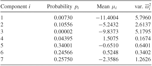
To demonstrate the adequacy of the approximation, Figure 12.12 shows the density function of ![]() (solid line) and that of the mixture of seven normals (dashed line) in Table 12.3. These densities are obtained using simulations with 100,000 observations. From the plot, the approximation by the mixture of seven normals is very good.
(solid line) and that of the mixture of seven normals (dashed line) in Table 12.3. These densities are obtained using simulations with 100,000 observations. From the plot, the approximation by the mixture of seven normals is very good.
Figure 12.12 Density functions of log(![]() ), solid line, and that of a mixture of seven normal distributions, dashed line. Results are based on 100,000 observations.
), solid line, and that of a mixture of seven normal distributions, dashed line. Results are based on 100,000 observations.

Why is it important to have a Gaussian state-space model? The answer is that such a Gaussian model enables us to draw the log volatility series ![]() jointly and efficiently. To see this, consider the following special Gaussian state-space model, where ηt and et are uncorrelated (i.e., no leverage effects):
jointly and efficiently. To see this, consider the following special Gaussian state-space model, where ηt and et are uncorrelated (i.e., no leverage effects):
where, as will be seen later, (ct, Ht) assumes the value ![]() of Table 12.3 for some i. For this special state-space model, we have the Kalman filter algorithm
of Table 12.3 for some i. For this special state-space model, we have the Kalman filter algorithm

where Vt = Var(vt) is the variance of the 1-step-ahead prediction error vt of yt given Ft−1 = (y1, … , yt−1), and zj|i and Σj|i are, respectively, the conditional expectation and variance of the state variable zj given Fi. See the Kalman filter discussion of Chapter 11.
Forward Filtering and Backward Sampling
Let ![]() be the joint conditional posterior distribution of
be the joint conditional posterior distribution of ![]() given the return data and other parameters, where for simplicity the parameters are omitted from the condition set. We can partition the distribution as
given the return data and other parameters, where for simplicity the parameters are omitted from the condition set. We can partition the distribution as
where the last equality holds because zt in Eq. (12.43) is a Markov process so that conditioned on zt+1, zt is independent of zt+j for j > 1.
From the Kalman filter in Eq. (12.45), we obtain that p(zn|Fn) is normal with mean zn|n and variance Σn|n. Next, consider the second term p(zn−1|zn, Fn) of Eq. (12.46). We have
12.47 ![]()
where vn = yn − yn|n−1 is the 1-step-ahead prediction error of yn. From the state-space model in Eqs. (12.43) and (12.44), zn−1 is independent of vn. Therefore,
12.48 ![]()
This is an important property because it implies that we can derive the posterior distribution p(zn−1|zn, Fn) from the joint distribution of (zn−1, zn) given Fn−1 via Theorem 11.1. First, the joint distribution is bivariate normal under the Gaussian assumption. Second, the conditional mean and covariance matrix of (zn−1, zn) given Fn−1 are readily available from the Kalman filter algorithm in Eq. (12.45). Specifically, we have
where the covariance is obtained by (i) multiplying zn−1 by Eq. (12.43) and (ii) taking conditional expectation. Note that all quantities involved in Eq. (12.49) are available from the Kalman filter. Consequently, by Theorem 11.1, we have
12.50 ![]()
where
![]()
Next, for the conditional posterior distribution p(zn−2|zn−1, Fn), we have
Consequently, we can obtain p(zn−2|zn−1, Fn) from the bivariate normal distribution of p(zn−2, zn−1|Fn−2) as before. In general, we have
![]()
Furthermore, from the Kalman filter, p(zt, zt+1|Ft) is bivariate normal as
12.51 ![]()
Consequently,
![]()
where
![]()
The prior derivation implies that we can draw the volatility series ![]() jointly by a recursive method using quantities readily available from the Kalman filter algorithm. That is, given the initial values z1|0 and Σ1|0, one uses the Kalman filter in Eq. (12.45) to process the return data forward, then applies the recursive backward method to draw a realization of the volatility series
jointly by a recursive method using quantities readily available from the Kalman filter algorithm. That is, given the initial values z1|0 and Σ1|0, one uses the Kalman filter in Eq. (12.45) to process the return data forward, then applies the recursive backward method to draw a realization of the volatility series ![]() . This scheme is referred to as forward filtering and backward sampling (FFBS); see Carter and Kohn (1994) and Frühwirth-Schnatter (1994). Because the volatility {zt} is serially correlated, drawing the series jointly is more efficient.
. This scheme is referred to as forward filtering and backward sampling (FFBS); see Carter and Kohn (1994) and Frühwirth-Schnatter (1994). Because the volatility {zt} is serially correlated, drawing the series jointly is more efficient.
Remark
The FFBS procedure applies to general linear Gaussian state-space models. The main idea is to make use of the Markov property of the model and the structure of the state transition equation so that
![]()
where ![]() denotes the state variable at time t and vj is the 1-step-ahead prediction error. This identity enables us to apply Theorem 11.27 to derive a recursive method to draw the state vectors jointly. □
denotes the state variable at time t and vj is the 1-step-ahead prediction error. This identity enables us to apply Theorem 11.27 to derive a recursive method to draw the state vectors jointly. □
Return to the estimation of the SV model. As in Eq. (12.42), let ![]() . To implement FFBS, one must determine ct and Ht of Eq. (12.44) so that the mixture of normals provides a good approximation to the distribution of
. To implement FFBS, one must determine ct and Ht of Eq. (12.44) so that the mixture of normals provides a good approximation to the distribution of ![]() . To this end, we augment the model with a series of independent indicator variables {It}, where It assumes a value in {1, … , 7} such that P(It = i) = pit with
. To this end, we augment the model with a series of independent indicator variables {It}, where It assumes a value in {1, … , 7} such that P(It = i) = pit with ![]() for each t. In practice, conditioned on {zt}, we can determine ct and Ht as follows. Let
for each t. In practice, conditioned on {zt}, we can determine ct and Ht as follows. Let
![]()
where μi and ![]() are the mean and standard error of the normal distributions given in Table 12.3 and Φ(·) denotes the cumulative distribution function of the standard normal random variable. These probabilities qit are the likelihood function of It given yt and zt. The probabilities pi of Table 12.3 form a prior distribution of It. Therefore, the posterior distribution of It is
are the mean and standard error of the normal distributions given in Table 12.3 and Φ(·) denotes the cumulative distribution function of the standard normal random variable. These probabilities qit are the likelihood function of It given yt and zt. The probabilities pi of Table 12.3 form a prior distribution of It. Therefore, the posterior distribution of It is
![]()
We can draw a realization of It using this posterior distribution. If the random draw is It = j, then we define ct = μj and ![]() . In summary, conditioned on the return data and other parameters of the model, we employ the approximate linear Gaussian state-space model in Eqs. (12.43) and (12.44) to draw jointly the log volatility series
. In summary, conditioned on the return data and other parameters of the model, we employ the approximate linear Gaussian state-space model in Eqs. (12.43) and (12.44) to draw jointly the log volatility series ![]() . It turns out that the resulting Gibbs sampling is efficient in estimating univariate stochastic volatility models.
. It turns out that the resulting Gibbs sampling is efficient in estimating univariate stochastic volatility models.
On the other hand, the square transformation involved in Eq. (12.42) fails to retain the correlation between ηt and ϵt if it exists, making the approximate state-space model in Eqs. (12.43) and (12.44) incapable of estimating the leverage effect. To overcome this inadequacy, Artigas and Tsay (2004) propose using a time-varying state-space model that maintains the leverage effect. Specifically, when ρ ≠ 0, we have
![]()
where ![]() is a normal random variable independent of ϵt and Var(
is a normal random variable independent of ϵt and Var(![]() ) =
) = ![]() . The state transition equation of Eq. (12.43) then becomes
. The state transition equation of Eq. (12.43) then becomes
![]()
Substituting ![]() , we obtain
, we obtain
12.52 ![]()
where ![]() . This is a nonlinear transition equation for the state variable zt. The Kalman filter in Eq. (12.45) is no longer applicable. To overcome this difficulty, Artigas and Tsay (2004) use a time-varying linear Kalman filter to approximate the system. Specifically, the last two equations of Eq. (12.45) are modified as
. This is a nonlinear transition equation for the state variable zt. The Kalman filter in Eq. (12.45) is no longer applicable. To overcome this difficulty, Artigas and Tsay (2004) use a time-varying linear Kalman filter to approximate the system. Specifically, the last two equations of Eq. (12.45) are modified as
12.53 ![]()
where ![]() is the first-order derivative of G(zt) evaluated at the smoothed state zt|t.
is the first-order derivative of G(zt) evaluated at the smoothed state zt|t.
Example 12.5
To demonstrate the FFBS procedure, we consider the monthly log returns of the S&P 500 index from January 1962 to November 2004 for 515 observations. This is a subseries of the data used in Example 12.3. See Figure 12.4 for time plots of the index and its log return. We consider two stochastic volatility models in the form:
12.54 ![]()
In model 1, {ϵt} and {ηt} are two independent Gaussian white noise series. That is, there is no leverage effect in the model. In model 2, we assume that corr(ϵt, et) = ρ, which denotes the leverage effect.
We estimate the models via the FFBS procedure using a program written in Matlab. The Gibbs sampling was run for 2000+8000 iterations with the first 2000 iterations as burn-ins. Table 12.4 gives the posterior means and standard errors of the parameter estimates. In particular, we have ![]() = − 0.39, which is close to the value commonly seen in the literature. Figure 12.13 shows the time plots of the posterior means of the estimated volatility. As expected, the two volatility series are very close. Compared with the results of Example 12.3, which uses a shorter series, the estimated volatility series exhibit similar patterns and are in the same magnitude. Note that the volatility shown in Figure 12.6 is conditional variance of percentage log returns whereas the volatility in Figure 12.13 is the conditional standard error of log returns.
= − 0.39, which is close to the value commonly seen in the literature. Figure 12.13 shows the time plots of the posterior means of the estimated volatility. As expected, the two volatility series are very close. Compared with the results of Example 12.3, which uses a shorter series, the estimated volatility series exhibit similar patterns and are in the same magnitude. Note that the volatility shown in Figure 12.6 is conditional variance of percentage log returns whereas the volatility in Figure 12.13 is the conditional standard error of log returns.
Figure 12.13 Estimated volatility of monthly log returns of S&P 500 index from January 1962 to November 2004 using stochastic volatility models: (a) with leverage effect and (b) without leverage effect.

Table 12.4 Estimation of Stochastic Volatility Model in Eq. (12.54) for Monthly Log Returns of S&P 500 Index from January 1962 to November 2004 Using Gibbs Sampling with FFBS Algorithma

a
The results are based on 2000+8000 iterations with the first 2000 iterations as burn-ins.