
8.3 Vector Moving-Average Models
A vector moving-average model of order q, or VMA(q), is in the form
where ![]() is a k-dimensional vector,
is a k-dimensional vector, ![]() are k × k matrices, and
are k × k matrices, and ![]() is the MA matrix polynomial in the back-shift operator B. Similar to the univariate case, VMA(q) processes are weakly stationary provided that the covariance matrix
is the MA matrix polynomial in the back-shift operator B. Similar to the univariate case, VMA(q) processes are weakly stationary provided that the covariance matrix ![]() of
of ![]() exists. Taking expectation of Eq. (8.23), we obtain that
exists. Taking expectation of Eq. (8.23), we obtain that ![]() . Thus, the constant vector
. Thus, the constant vector ![]() is the mean vector of
is the mean vector of ![]() for a VMA model.
for a VMA model.
Let ![]() be the mean-corrected VAR(q) process. Then using Eq. (8.23) and the fact that
be the mean-corrected VAR(q) process. Then using Eq. (8.23) and the fact that ![]() has no serial correlations, we have
has no serial correlations, we have
1. Cov(![]() ) =
) = ![]() .
.
2. ![]() .
.
3. ![]() if ℓ > q.
if ℓ > q.
4. ![]() if 1 ≤ ℓ ≤ q, where
if 1 ≤ ℓ ≤ q, where ![]() .
.
Since ![]() for ℓ > q, the cross-correlation matrices (CCMs) of a VMA(q) process
for ℓ > q, the cross-correlation matrices (CCMs) of a VMA(q) process ![]() satisfy
satisfy
8.24 ![]()
Therefore, similar to the univariate case, the sample CCMs can be used to identify the order of a VMA process.
To better understand the VMA processes, let us consider the bivariate MA(1) model
where, for simplicity, the subscript of ![]() is removed. This model can be written explicitly as
is removed. This model can be written explicitly as
8.26 ![]()
It says that the current return series ![]() only depends on the current and past shocks. Therefore, the model is a finite-memory model.
only depends on the current and past shocks. Therefore, the model is a finite-memory model.
Consider the equation for r1t in Eq. (8.27). The parameter Θ12 denotes the linear dependence of r1t on a2, t−1 in the presence of a1, t−1. If Θ12 = 0, then r1t does not depend on the lagged values of a2t and, hence, the lagged values of r2t. Similarly, if Θ21 = 0, then r2t does not depend on the past values of r1t. The off-diagonal elements of ![]() thus show the dynamic dependence between the component series. For this simple VMA(1) model, we can classify the relationships between r1t and r2t as follows:
thus show the dynamic dependence between the component series. For this simple VMA(1) model, we can classify the relationships between r1t and r2t as follows:
1. They are uncoupled series if Θ12 = Θ21 = 0.
2. There is a unidirectional dynamic relationship from r1t to r2t if ![]() = 0, but Θ21 ≠ 0. The opposite unidirectional relationship holds if Θ21 = 0, but Θ12 ≠ 0.
= 0, but Θ21 ≠ 0. The opposite unidirectional relationship holds if Θ21 = 0, but Θ12 ≠ 0.
3. There is a feedback relationship between r1t and r2t if Θ12 ≠ 0 and Θ21 ≠ 0.
Finally, the concurrent correlation between rit is the same as that between ait. The previous classification can be generalized to a VMA(q) model.
Estimation
Unlike the VAR models, estimation of VMA models is much more involved; see Hillmer and Tiao (1979), Lütkepohl (2005), and the references therein. For the likelihood approach, there are two methods available. The first is the conditional-likelihood method that assumes that ![]() for t ≤ 0. The second is the exact-likelihood method that treats
for t ≤ 0. The second is the exact-likelihood method that treats ![]() with t ≤ 0 as additional parameters of the model. To gain some insight into the problem of estimation, we consider the VMA(1) model in Eq. (8.25). Suppose that the data are
with t ≤ 0 as additional parameters of the model. To gain some insight into the problem of estimation, we consider the VMA(1) model in Eq. (8.25). Suppose that the data are ![]() and
and ![]() is multivariate normal. For a VMA(1) model, the data depend on
is multivariate normal. For a VMA(1) model, the data depend on ![]() .
.
8.3.1.1 Conditional MLE
The conditional-likelihood method assumes that ![]() =
= ![]() . Under such an assumption and rewriting the model as
. Under such an assumption and rewriting the model as ![]() , we can compute the shock
, we can compute the shock ![]() recursively as
recursively as
![]()
Consequently, the likelihood function of the data becomes
![]()
which can be evaluated to obtain the parameter estimates.
8.3.1.2 Exact MLE
For the exact-likelihood method, ![]() is an unknown vector that must be estimated from the data to evaluate the likelihood function. For simplicity, let
is an unknown vector that must be estimated from the data to evaluate the likelihood function. For simplicity, let ![]() be the mean-corrected series. Using
be the mean-corrected series. Using ![]() and Eq. (8.25), we have
and Eq. (8.25), we have
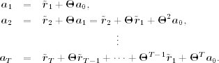
By repeated substitutions, ![]() is related to all
is related to all ![]() as
as
Thus, ![]() is a linear function of the data if
is a linear function of the data if ![]() and
and ![]() are given. This result enables us to estimate
are given. This result enables us to estimate ![]() using the data and initial estimates of
using the data and initial estimates of ![]() and
and ![]() . More specifically, given
. More specifically, given ![]() ,
, ![]() , and the data, we can define
, and the data, we can define
![]()
Equation (8.29) can then be rewritten as

This is in the form of a multiple linear regression with parameter vector ![]() , even though the covariance matrix
, even though the covariance matrix ![]() of
of ![]() may not be a diagonal matrix. If initial estimate of
may not be a diagonal matrix. If initial estimate of ![]() is also available, one can premultiply each equation of the prior system by
is also available, one can premultiply each equation of the prior system by ![]() , which is the square root matrix of
, which is the square root matrix of ![]() . The resulting system is indeed a multiple linear regression, and the ordinary least-squares method can be used to obtain an estimate of
. The resulting system is indeed a multiple linear regression, and the ordinary least-squares method can be used to obtain an estimate of ![]() . Denote the estimate by
. Denote the estimate by ![]() .
.
Using the estimate ![]() , we can compute the shocks
, we can compute the shocks ![]() recursively as
recursively as
![]()
This recursion is a linear transformation from ![]() to
to ![]() , from which we can (a) obtain the joint distribution of
, from which we can (a) obtain the joint distribution of ![]() and the data, and (2) integrate out
and the data, and (2) integrate out ![]() to derive the exact-likelihood function of the data. The resulting likelihood function can then be evaluated to obtain the exact ML estimates. For details, see Hillmer and Tiao (1979).
to derive the exact-likelihood function of the data. The resulting likelihood function can then be evaluated to obtain the exact ML estimates. For details, see Hillmer and Tiao (1979).
In summary, the exact-likelihood method works as follows. Given initial estimates of ![]() ,
, ![]() , and
, and ![]() , one uses Eq. (8.29) to derive an estimate of
, one uses Eq. (8.29) to derive an estimate of ![]() . This estimate is in turn used to compute
. This estimate is in turn used to compute ![]() recursively using Eq. (8.28) and starting with
recursively using Eq. (8.28) and starting with ![]() . The resulting
. The resulting ![]() are then used to evaluate the exact-likelihood function of the data to update the estimates of
are then used to evaluate the exact-likelihood function of the data to update the estimates of ![]() ,
, ![]() , and
, and ![]() . The whole process is then repeated until the estimates converge. This iterative method to evaluate the exact-likelihood function applies to the general VMA(q) models.
. The whole process is then repeated until the estimates converge. This iterative method to evaluate the exact-likelihood function applies to the general VMA(q) models.
From the previous discussion, the exact-likelihood method requires more intensive computation than the conditional-likelihood approach does. But it provides more accurate parameter estimates, especially when some eigenvalues of ![]() are close to 1 in modulus. Hillmer and Tiao (1979) provide some comparison between the conditional- and exact-likelihood estimations of VMA models. In multivariate time series analysis, the exact maximum-likelihood method becomes important if one suspects that the data might have been overdifferenced. Overdifferencing may occur in many situations (e.g., differencing individual components of a cointegrated system; see discussion later on cointegration).
are close to 1 in modulus. Hillmer and Tiao (1979) provide some comparison between the conditional- and exact-likelihood estimations of VMA models. In multivariate time series analysis, the exact maximum-likelihood method becomes important if one suspects that the data might have been overdifferenced. Overdifferencing may occur in many situations (e.g., differencing individual components of a cointegrated system; see discussion later on cointegration).
In summary, building a VMA model involves three steps: (a) Use the sample cross-correlation matrices to specify the order q—for a VMA(q) model, ![]() for ℓ > q; (b) estimate the specified model by using either the conditional- or exact-likelihood method—the exact method is preferred when the sample size is not large; and (c) the fitted model should be checked for adequacy [e.g., applying the Qk(m) statistics to the residual series]. Finally, forecasts of a VMA model can be obtained by using the same procedure as a univariate MA model.
for ℓ > q; (b) estimate the specified model by using either the conditional- or exact-likelihood method—the exact method is preferred when the sample size is not large; and (c) the fitted model should be checked for adequacy [e.g., applying the Qk(m) statistics to the residual series]. Finally, forecasts of a VMA model can be obtained by using the same procedure as a univariate MA model.
Example 8.5
Consider again the bivariate series of monthly log returns in percentages of IBM stock and the S&P 500 index from January 1926 to December 2008. Since significant cross correlations occur mainly at lags 1, 2, 3 and 5, we employ the VMA(5) model
for the data. Table 8.6 shows the estimation results of the model. The Qk(m) statistics for the residuals of the simplified model give Q2(4) = 16.00 and Q2(8) = 29.46. Compared with chi-squared distributions with 10 and 26 degrees of freedom, the p values of these statistics are 0.10 and 0.291, respectively. Thus, the model is adequate at the 5% significance level.
From Table 8.6, we make the following observations:
1. The difference between conditional- and exact-likelihood estimates is small for this particular example. This is not surprising because the sample size is not small and, more important, the dynamic structure of the data is weak.
2. The VMA(5) model provides essentially the same dynamic relationship for the series as that of the VAR(5) model in Example 8.4. The monthly log return of IBM stock depends on the previous returns of the S&P 500 index. The market return, in contrast, does not depend on lagged returns of IBM stock. In other words, the dynamic structure of the data is driven by the market return, not by the IBM return. The concurrent correlation between the two returns remains strong, however.
Table 8.6 Estimation Results for Monthly Log Returns of IBM Stock and S&P 500 Index Using the Vector Moving-Average Model in Eq. (8.30)a

aThe sample period is from January 1926 to December 2008. The residual covariance matrix is not shown as it is similar to that in Table 8.4