8.2 Vector Autoregressive Models

A simple vector model useful in modeling asset returns is the vector autoregressive (VAR) model. A multivariate time series is a VAR process of order 1, or VAR(1) for short, if it follows the model

8.8

where is a k-dimensional vector, is a k × k matrix, and is a sequence of serially uncorrelated random vectors with mean zero and covariance matrix . In application, the covariance matrix is required to be positive definite; otherwise, the dimension of can be reduced. In the literature, it is often assumed that is multivariate normal.

Consider the bivariate case [i.e., k = 2, , and ]. The VAR(1) model consists of the following two equations:

where Φij is the (i, j)th element of and ϕi0 is the ith element of . Based on the first equation, Φ12 denotes the linear dependence of r1t on r2, t−1 in the presence of r1, t−1. Therefore, Φ12 is the conditional effect of r2, t−1 on r1t given r1, t−1. If Φ12 = 0, then r1t does not depend on r2, t−1, and the model shows that r1t only depends on its own past. Similarly, if Φ21 = 0, then the second equation shows that r2t does not depend on r1, t−1 when r2, t−1 is given.

Consider the two equations jointly. If Φ12 = 0 and Φ21 ≠ 0, then there is a unidirectional relationship from r1t to r2t. If Φ12 = Φ21 = 0, then r1t and r2t are uncoupled. If Φ12 ≠ 0 and Φ21 ≠ 0, then there is a feedback relationship between the two series.

8.2.1 Reduced and Structural Forms

In general, the coefficient matrix of Eq. (8.8) measures the dynamic dependence of . The concurrent relationship between r1t and r2t is shown by the off-diagonal element σ12 of the covariance matrix of . If σ12 = 0, then there is no concurrent linear relationship between the two component series. In the econometric literature, the VAR(1) model in Eq. (8.8) is called a reduced-form model because it does not show explicitly the concurrent dependence between the component series. If necessary, an explicit expression involving the concurrent relationship can be deduced from the reduced-form model by a simple linear transformation. Because is positive definite, there exists a lower triangular matrix with unit diagonal elements and a diagonal matrix such that = ; see Appendix A on Cholesky decomposition. Therefore, .

Define . Then

Since is a diagonal matrix, the components of are uncorrelated. Multiplying from the left to model (8.8), we obtain

8.9

where is a k-dimensional vector and = is a k × k matrix. Because of the special matrix structure, the kth row of is in the form (wk1, wk2, … , wk, k−1, 1). Consequently, the kth equation of model (8.9) is

8.10

where is the kth element of and is the (k, i)th element of . Because bkt is uncorrelated with bit for 1 ≤ i < k, Eq. (8.10) shows explicitly the concurrent linear dependence of rkt on rit, where 1 ≤ i ≤ k − 1. This equation is referred to as a structural equation for rkt in the econometric literature.

For any other component rit of , we can rearrange the VAR(1) model so that rit becomes the last component of . The prior transformation method can then be applied to obtain a structural equation for rit. Therefore, the reduced-form model (8.8) is equivalent to the structural form used in the econometric literature. In time series analysis, the reduced-form model is commonly used for two reasons. The first reason is ease in estimation. The second and main reason is that the concurrent correlations cannot be used in forecasting.

8.2.2 Stationarity Condition and Moments of a VAR(1) Model

Assume that the VAR(1) model in Eq. (8.8) is weakly stationary. Taking expectation of the model and using = , we obtain

Since is time invariant, we have

provided that the matrix is nonsingular, where is the k × k identity matrix.

Using , the VAR(1) model in Eq. (8.8) can be written as

Let be the mean-corrected time series. Then the VAR(1) model becomes

8.11

This model can be used to derive properties of a VAR(1) model. By repeated substitutions, we can rewrite Eq. (8.11) as

This expression shows several characteristics of a VAR(1) process. First, since is serially uncorrelated, it follows that Cov() = . In fact, is not correlated with for all ℓ > 0. For this reason, is referred to as the shock or innovation of the series at time t. It turns out that, similar to the univariate case, is uncorrelated with the past value (j > 0) for all time series models. Second, postmultiplying the expression by , taking expectation, and using the fact of no serial correlations in the process, we obtain Cov() = . Third, for a VAR(1) model, depends on the past innovation with coefficient matrix . For such dependence to be meaningful, must converge to zero as j → ∞. This means that the k eigenvalues of must be less than 1 in modulus; otherwise, will either explode or converge to a nonzero matrix as j → ∞. As a matter of fact, the requirement that all eigenvalues of are less than 1 in modulus is the necessary and sufficient condition for weak stationarity of provided that the covariance matrix of

exists. Notice that this stationarity condition reduces to that of the univariate AR(1) case in which the condition is |ϕ| < 1. Furthermore, because

the eigenvalues of are the inverses of the zeros of the determinant . Thus, an equivalent sufficient and necessary condition for stationarity of is that all zeros of the determinant

are greater than one in modulus; that is, all zeros are outside the unit circle in the complex plane. Fourth, using the expression, we have

where it is understood that , the k × k identity matrix.

Postmultiplying to Eq. (8.11), taking expectation, and using the result Cov() = for j > 0, we obtain

Therefore,

8.12

where is the lag-j cross-covariance matrix of

. Again this result is a generalization of that of a univariate AR(1) process. By repeated substitutions, Eq. (8.12) shows that

Pre- and postmultiplying Eq. (8.12) by

, we obtain

where . Consequently, the CCM of a VAR(1) model satisfies

8.2.3 Vector AR(p) Models

The generalization of VAR(1) to VAR(p) models is straightforward. The time series follows a VAR(p) model if it satisfies

8.13

where and are defined as before, and are k × k matrices. Using the back-shift operator B, the VAR(p) model can be written as

where is the k × k identity matrix. This representation can be written in a compact form as

where is a matrix polynomial. If is weakly stationary, then we have

provided that the inverse exists. Let . The VAR(p) model becomes

8.14

Using this equation and the same techniques as those for VAR(1) models, we obtain that

• Cov() = , the covariance matrix of .
• Cov() = for ℓ > 0.
• for ℓ > 0.

The last property is called the moment equations of a VAR(p) model. It is a multivariate version of the Yule–Walker equation of a univariate AR(p) model. In terms of CCM, the moment equations become

where .

A simple approach to understanding properties of the VAR(p) model in Eq. (8.13) is to make use of the results of the VAR(1) model in Eq. (8.8). This can be achieved by transforming the VAR(p) model of into a kp-dimensional VAR(1) model. Specifically, let and be two kp-dimensional processes. The mean of is zero and the covariance matrix of is a kp × kp matrix with zero everywhere except for the lower right corner, which is . The VAR(p) model for can then be written in the form

8.15

where is a kp × kp matrix given by

where and are the k × k zero matrix and identity matrix, respectively. In the literature, is called the companion matrix of the matrix polynomial .

Equation (8.15) is a VAR(1) model for , which contains as its last k components. The results of a VAR(1) model shown in the previous section can now be used to derive properties of the VAR(p) model via Eq. (8.15). For example, from the definition, is weakly stationary if and only if is weakly stationary. Therefore, the necessary and sufficient condition of weak stationarity for the VAR(p) model in Eq. (8.13) is that all eigenvalues of in Eq. (8.15) are less than 1 in modulus. It is easy to show that . Therefore, similar to the VAR(1) case, the necessary and sufficient condition is equivalent to all zeros of the determinant being outside the unit circle.

Of particular relevance to financial time series analysis is the structure of the coefficient matrices of a VAR(p) model. For instance, if the (i, j)th element Φij(ℓ) of is zero for all ℓ, then rit does not depend on the past values of rjt. The structure of the coefficient matrices thus provides information on the lead–lag relationship between the components of .

8.2.4 Building a VAR(p) Model

We continue to use the iterative procedure of order specification, estimation, and model checking to build a vector AR model for a given time series. The concept of partial autocorrelation function of a univariate series can be generalized to specify the order p of a vector series. Consider the following consecutive VAR models:

8.16

Parameters of these models can be estimated by the ordinary least-squares (OLS) method. This is called the multivariate linear regression estimation in multivariate statistical analysis; see Johnson and Wichern (1998).

For the ith equation in Eq. (8.16), let be the OLS estimate of and be the estimate of , where the superscript (i) is used to denote that the estimates are for a VAR(i) model. Then the residual is

For i = 0, the residual is defined as , where is the sample mean of . The residual covariance matrix is defined as

8.17

To specify the order p, one can test the hypothesis versus the alternative hypothesis sequentially for ℓ = 1, 2, … . For example, using the first equation in Eq. (8.16), we can test the hypothesis versus the alternative hypothesis . The test statistic is

where is defined in Eq. (8.17) and denotes the determinant of the matrix . Under some regularity conditions, the test statistic M(1) is asymptotically a chi-squared distribution with k2 degrees of freedom; see Tiao and Box (1981).

In general, we use the ith and (i − 1)th equations in Eq. (8.16) to test versus ; that is, testing a VAR(i) model versus a VAR(i − 1) model. The test statistic is

8.18

Asymptotically, M(i) is distributed as a chi-squared distribution with k2 degrees of freedom.

Alternatively, one can use the Akaike information criterion (AIC) or its variants to select the order p. Assume that is multivariate normal and consider the ith equation in Eq. (8.16). One can estimate the model by the maximum-likelihood (ML) method. For AR models, the OLS estimates and are equivalent to the (conditional) ML estimates. However, there are differences between the estimates of . The ML estimate of is

8.19

The AIC of a VAR(i) model under the normality assumption is defined as

For a given vector time series, one selects the AR order p such that , where p0 is a prespecified positive integer.

Other information criteria available for VAR(i) models are

The HQ criterion is proposed by Hannan and Quinn (1979).

Example 8.4

Assuming that the bivariate series of monthly log returns of IBM stock and the S&P 500 index discussed in Example 8.1 follows a VAR model, we apply the M(i) statistics and AIC to the data. Table 8.3 shows the results of these statistics. Both statistics indicate that a VAR(5) model might be adequate for the data. The M(i) statistics are marginally significant at lags 1, 3, and 5 at the 5% level. The minimum of AIC occurs at order 5. For this particular instance, the M(i) statistic is only marginally significant at the 1% level when i = 2, confirming the previous observation that the dynamic linear dependence between the two return series is weak.

Table 8.3 Order Specification Statistics for Monthly Log Returns of IBM Stock and S&P 500 Index from January 1926 to December 2008a

aThe 5% and 1% critical values of a chi-squared distribution with 4 degrees of freedom are 9.5 and 13.3.

8.2.4.1 Estimation and Model Checking

For a specified VAR model, one can estimate the parameters using either the OLS method or the ML method. The two methods are asymptotically equivalent. Under some regularity conditions, the estimates are asymptotically normal; see Reinsel (1993). A fitted model should then be checked carefully for any possible inadequacy. The Qk(m) statistic can be applied to the residual series to check the assumption that there are no serial or cross correlations in the residuals. For a fitted VAR(p) model, the Qk(m) statistic of the residuals is asymptotically a chi-squared distribution with k2m − g degrees of freedom, where g is the number of estimated parameters in the AR coefficient matrices; see Lütkepohl (2005).

Example 8.4(Continued)

Table 8.4(a) shows the estimation results of a VAR(5) model for the bivariate series of monthly log returns of IBM stock and the S&P 500 index. The specified model is in the form

8.20

where the first component of denotes IBM stock returns. For this particular instance, we do not use AR coefficient matrix at lag 4 because of the weak serial dependence of the data. In general, when the M(i) statistics and the AIC criterion specify a VAR(5) model, all five AR lags should be used. Table 8.4(b) shows the estimation results after some statistically insignificant parameters are set to zero. The Qk(m) statistics of the residual series for the fitted model in Table 8.4(b) give Q2(4) = 16.64 and Q2(8) = 31.55. Since the fitted VAR(5) model has six parameters in the AR coefficient matrices, these two Qk(m) statistics are distributed asymptotically as a chi-squared distribution with degrees of freedom 10 and 26, respectively. The p-values of the test statistics are 0.083 and 0.208, and hence the fitted model is adequate at the 5% significance level. As shown by the univariate analysis, the return series are likely to have conditional heteroscedasticity. We discuss multivariate volatility in Chapter 10.

Table 8.4 Estimation Results of a VAR(5) Model for the Monthly Log Returns, in Percentages, of IBM Stock and S&P 500 Index from January 1926 to December 2008

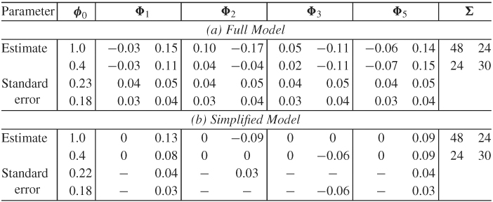
From the fitted model in Table 8.4(b), we make the following observations: (a) The concurrent correlation coefficient between the two innovational series is , which, as expected, is close to the sample correlation coefficient between r1t and r2t. (b) The two log return series have positive and significant means, implying that the log prices of the two series had an upward trend over the data span. (c) The model shows that

Consequently, at the 5% significance level, there is a unidirectional dynamic relationship from the monthly S&P 500 index return to the IBM return. If the S&P 500 index represents the U.S. stock market, then IBM return is affected by the past movements of the market. However, past movements of IBM stock returns do not significantly affect the U.S. market, even though the two returns have substantial concurrent correlation. Finally, the fitted model can be written as

indicating that SP5t is the driving factor of the bivariate series.

8.2.4.2 Forecasting

Treating a properly built model as the true model, one can apply the same techniques as those in the univariate analysis to produce forecasts and standard deviations of the associated forecast errors. For a VAR(p) model, the 1-step-ahead forecast at the time origin h is , and the associated forecast error is = . The covariance matrix of the forecast error is . For 2-step-ahead forecasts, we substitute by its forecast to obtain

and the associated forecast error is

The covariance matrix of the forecast error is . If is weakly stationary, then the ℓ-step-ahead forecast converges to its mean vector as the forecast horizon ℓ increases and the covariance matrix of its forecast error converges to the covariance matrix of .

Table 8.5 provides 1-step- to 6-step-ahead forecasts of the monthly log returns, in percentages, of IBM stock and the S&P 500 index at the forecast origin h = 996. These forecasts are obtained by the refined VAR(5) model in Table 8.4(b). As expected, the standard errors of the forecasts converge to the sample standard errors 7.03 and 5.53, respectively, for the two log return series.

Table 8.5 Forecasts of a VAR(5) Model for Monthly Log Returns, in Percentages, of IBM Stock and S&P 500 Index: Forecast Origin Is December 2008

In summary, building a VAR model involves three steps: (a) Use the test statistic M(i) or some information criterion to identify the order, (b) estimate the specified model by using the least-squares method and, if necessary, reestimate the model by removing statistically insignificant parameters, and (c) use the Qk(m) statistic of the residuals to check the adequacy of a fitted model. Other characteristics of the residual series, such as conditional heteroscedasticity and outliers, can also be checked. If the fitted model is adequate, then it can be used to obtain forecasts and make inference concerning the dynamic relationship between the variables.

We used SCA to perform the analysis in this section. The commands used include miden, mtsm, mest, and mfore, where the prefix m stands for multivariate. Details of the commands and output are shown below.

8.2.4.3 SCA Demonstration

Output has been edited and % denotes explanation in the following:

8.2.5 Impulse Response Function

Similar to the univariate case, a VAR(p) model can be written as a linear function of the past innovations, that is,

8.21

where = provided that the inverse exists, and the coefficient matrices can be obtained by equating the coefficients of Bi in the equation

where is the identity matrix. This is a moving-average representation of with the coefficient matrix being the impact of the past innovation on . Equivalently, is the effect of on the future observation . Therefore, is often referred to as the impulse response function of . However, since the components of are often correlated, the interpretation of elements in of Eq. (8.21) is not straightforward. To aid interpretation, one can use the Cholesky decomposition mentioned earlier to transform the innovations so that the resulting components are uncorrelated. Specifically, there exists a lower triangular matrix such that , where is a diagonal matrix and the diagonal elements of are unity. See Eq. (8.9). Let . Then, Cov() = so that the elements bjt are uncorrelated. Rewrite Eq. (8.21) as

8.22

where and . The coefficient matrices are called the impulse response function of with respect to the orthogonal innovations . Specifically, the (i, j)th element of ; that is, , is the impact of bj, t on the future observation ri, t+ℓ. In practice, one can further normalize the orthogonal innovation such that the variance of bit is one. A weakness of the above orthogonalization is that the result depends on the ordering of the components of . In particular, b1t = a1t so that a1t is not transformed. Different orderings of the components of may lead to different impulse response functions. Interpretation of the impulse response function is, therefore, associated with the innovation series .

Both SCA and S-Plus enable one to obtain the impulse response function of a fitted VAR model. To demonstrate analysis of VAR models in S-Plus, we again use the monthly log return series of IBM stock and the S&P 500 index of Example 8.1. For details of S-Plus commands, see Zivot and Wang (2003).

8.2.5.1 S-Plus Demonstration

The following output has been edited and % denotes explanation:

The AIC selects a VAR(5) model as before, but BIC selects a VAR(1) model. For simplicity, we shall use VAR(1) specification in the demonstration. Note that different normalizations are used between the two packages so that the values of information criteria appear to be different; see the AIC in Table 8.3. This is not important because normalization does not affect order selection. Turn to estimation.

The fitted model is

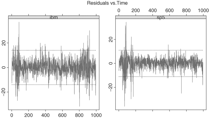
Based on t statistics of the coefficient estimates, only the lagged variable SP5t−1 is informative in both equations. Figure 8.5 shows the time plots of the two residual series, where the two horizontal lines indicate the two standard error limits. As expected, there exist clusters of outlying observations.

Figure 8.5 Residual plots of fitting a VAR(1) model to the monthly log returns, in percentages, of IBM stock and S&P 500 index. Sample period is from January 1926 to December 2008.

Next, we compute 1-step- to 6-step-ahead forecasts and the impulse response function of the fitted VAR(1) model when the IBM stock return is the first component of . Compared with those of a VAR(5) model in Table 8.5, the forecasts of the VAR(1) model converge faster to the sample mean of the series.

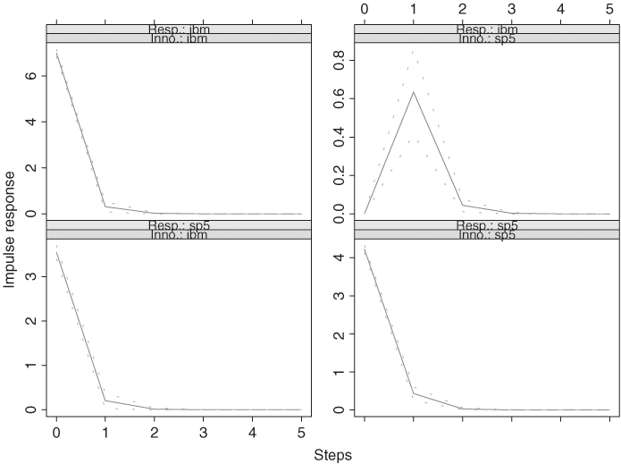
Figure 8.6 shows the forecasts and their pointwise 95% confidence intervals along with the last 12 data points of the series. Figure 8.7 shows the impulse response functions of the fitted VAR(1) model where the IBM stock return is the first component of . Since the dynamic dependence of the returns is weak, the impulse response functions exhibit simple patterns and decay quickly.

Figure 8.6 Forecasting plots of fitted VAR(1) model to monthly log returns, in percentages, of IBM stock and S&P 500 index. Sample period is from January 1926 to December 2008.

Figure 8.7 Plots of impulse response functions of orthogonal innovations for fitted VAR(1) model to monthly log returns, in percentages, of IBM stock and S&P 500 index. Sample period is from January 1926 to December 2008.