
Univariate ARMA models can also be generalized to handle vector time series. The resulting models are called VARMA models. The generalization, however, encounters some new issues that do not occur in developing VAR and VMA models. One of the issues is the identifiability problem. Unlike the univariate ARMA models, VARMA models may not be uniquely defined. For example, the VMA(1) model
![]()
is identical to the VAR(1) model
![]()
The equivalence of the two models can easily be seen by examining their component models. For the VMA(1) model, we have
![]()
For the VAR(1) model, the equations are
![]()
From the model for r2t, we have r2, t−1 = a2, t−1. Therefore, the models for r1t are identical. This type of identifiability problem is harmless because either model can be used in a real application.
Another type of identifiability problem is more troublesome. Consider the VARMA(1,1) model
![]()
This model is identical to the VARMA(1,1) model
![]()
for any nonzero ω and η. In this particular instance, the equivalence occurs because we have r2t = a2t in both models. The effects of the parameters ω and η on the system cancel out between AR and MA parts of the second model. Such an identifiability problem is serious because, without proper constraints, the likelihood function of a vector ARMA(1,1) model for the data is not uniquely defined, resulting in a situation similar to the exact multicollinearity in a regression analysis. This type of identifiability problem can occur in a vector model even if none of the components is a white noise series.
These two simple examples highlight the new issues involved in the generalization to VARMA models. Building a VARMA model for a given data set thus requires some attention. In the time series literature, methods of structural specification have been proposed to overcome the identifiability problem; see Tiao and Tsay (1989), Tsay (1991), and the references therein. We do not discuss the detail of structural specification here because VAR and VMA models are sufficient in most financial applications. When VARMA models are used, only lower order models are entertained [e.g., a VARMA(1,1) or VARMA(2,1) model] especially when the time series involved are not seasonal.
A VARMA(p, q) model can be written as
![]()
where ![]() and
and ![]() are two k × k matrix polynomials. We assume that the two matrix polynomials have no left common factors; otherwise, the model can be simplified. The necessary and sufficient condition of weak stationarity for
are two k × k matrix polynomials. We assume that the two matrix polynomials have no left common factors; otherwise, the model can be simplified. The necessary and sufficient condition of weak stationarity for ![]() is the same as that for the VAR(p) model with matrix polynomial
is the same as that for the VAR(p) model with matrix polynomial ![]() . For v > 0, the (i, j)th elements of the coefficient matrices
. For v > 0, the (i, j)th elements of the coefficient matrices ![]() and
and ![]() measure the linear dependence of r1t on rj, t−v and aj, t−v, respectively. If the (i, j)th element is zero for all AR and MA coefficient matrices, then rit does not depend on the lagged values of rjt. However, the converse proposition does not hold in a VARMA model. In other words, nonzero coefficients at the (i, j)th position of AR and MA matrices may exist even when rit does not depend on any lagged value of rjt.
measure the linear dependence of r1t on rj, t−v and aj, t−v, respectively. If the (i, j)th element is zero for all AR and MA coefficient matrices, then rit does not depend on the lagged values of rjt. However, the converse proposition does not hold in a VARMA model. In other words, nonzero coefficients at the (i, j)th position of AR and MA matrices may exist even when rit does not depend on any lagged value of rjt.
To illustrate, consider the following bivariate model
![]()
Here the necessary and sufficient conditions for the existence of a unidirectional dynamic relationship from r1t to r2t are
but
![]()
These conditions can be obtained as follows. Letting
![]()
be the determinant of the AR matrix polynomial and premultiplying the model by the matrix
![]()
we can rewrite the bivariate model as

Consider the equation for r1t. The first condition in Eq. (8.33) shows that r1t does not depend on any past value of a2t or r2t. From the equation for r2t, the second condition in Eq. (8.33) implies that r2t indeed depends on some past values of a1t. Based on Eq. (8.33), Θ12(B) = Φ12(B) = 0 is a sufficient, but not necessary, condition for the unidirectional relationship from r1t to r2t.
Estimation of a VARMA model can be carried out by either the conditional or exact maximum-likelihood method. The Qk(m) statistic continues to apply to the residual series of a fitted model, but the degrees of freedom of its asymptotic chi-squared distribution are k2m − g, where g is the number of estimated parameters in both the AR and MA coefficient matrices.
Example 8.6
To demonstrate VARMA modeling, we consider two U.S. monthly interest rate series. The first series is the 1-year Treasury constant maturity rate, and the second series is the 3-year Treasury constant maturity rate. The data are obtained from the Federal Reserve Bank of St. Louis, and the sampling period is from April 1953 to January 2001. There are 574 observations. To ensure the positiveness of U.S. interest rates, we analyze the log series. Figure 8.8 shows the time plots of the two log interest rate series. The solid line denotes the 1-year maturity rate. The two series moved closely in the sampling period.
Figure 8.8 Time plots of log U.S. monthly interest rates from April 1953 to January 2001. Solid line denotes 1-year Treasury constant maturity rate and dashed line denotes 3-year rate.

The M(i) statistics and AIC criterion specify a VAR(4) model for the data. However, we employ a VARMA(2,1) model because the two models provide similar fits. Table 8.7 shows the parameter estimates of the VARMA(2,1) model obtained by the exact-likelihood method. We removed the insignificant parameters and reestimated the simplified model. The residual series of the fitted model has some minor serial and cross correlations at lags 7 and 11. Figure 8.9 shows the residual plots and indicates the existence of some outlying data points. The model can be further improved, but it seems to capture the dynamic structure of the data reasonably well.
Figure 8.9 Residual plots for log U.S. monthly interest rate series of Example 8.6. Fitted model is VARMA(2,1): (a) 1-year rate and (b) 3-year rate.

Table 8.7 Parameter Estimates of VARMA(2,1) Model for Two Monthly U.S. Interest Rate Series Based on Exact-Likelihood Method
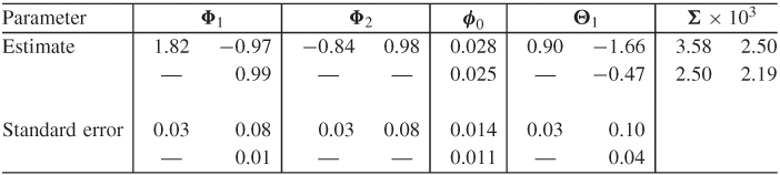
The final VARMA(2,1) model shows some interesting characteristics of the data. First, the interest rate series are highly contemporaneously correlated. The concurrent correlation coefficient is ![]() = 0.893. Second, there is a unidirectional linear relationship from the 3-year rate to the 1-year rate because the (2, 1)th elements of all AR and MA matrices are zero, but some (1, 2)th element is not zero. As a matter of fact, the model in Table 8.7 shows that
= 0.893. Second, there is a unidirectional linear relationship from the 3-year rate to the 1-year rate because the (2, 1)th elements of all AR and MA matrices are zero, but some (1, 2)th element is not zero. As a matter of fact, the model in Table 8.7 shows that

where rit is the log series of i-year interest rate and ait is the corresponding shock series. Therefore, the 3-year interest rate does not depend on the past values of the 1-year rate, but the 1-year rate depends on the past values of the 3-year rate. Third, the two interest rate series appear to be unit-root nonstationary. Using the back-shift operator B, the model can be rewritten approximately as
![]()
Finally, the SCA commands used in the analysis are given in Appendix C.
8.4.1 Marginal Models of Components
Given a vector model for ![]() , the implied univariate models for the components rit are the marginal models. For a k-dimensional ARMA(p, q) model, the marginal models are ARMA[kp, (k − 1)p + q]. This result can be obtained in two steps. First, the marginal model of a VMA(q) model is univariate MA(q). Assume that
, the implied univariate models for the components rit are the marginal models. For a k-dimensional ARMA(p, q) model, the marginal models are ARMA[kp, (k − 1)p + q]. This result can be obtained in two steps. First, the marginal model of a VMA(q) model is univariate MA(q). Assume that ![]() is a VMA(q) process. Because the cross-correlation matrix of
is a VMA(q) process. Because the cross-correlation matrix of ![]() vanishes after lag q (i.e.,
vanishes after lag q (i.e., ![]() =
= ![]() for ℓ > q), the ACF of rit is zero beyond lag q. Therefore, rit is an MA process and its univariate model is in the form
for ℓ > q), the ACF of rit is zero beyond lag q. Therefore, rit is an MA process and its univariate model is in the form ![]() , where {bit} is a sequence of uncorrelated random variables with mean zero and variance
, where {bit} is a sequence of uncorrelated random variables with mean zero and variance ![]() . The parameters θi, j and σib are functions of the parameters of the VMA model for
. The parameters θi, j and σib are functions of the parameters of the VMA model for ![]() .
.
The second step to obtain the result is to diagonalize the AR matrix polynomial of a VARMA(p, q) model. For illustration, consider the bivariate AR(1) model
![]()
Premultiplying the model by the matrix polynomial
![]()
we obtain
![]()
The left-hand side of the prior equation shows that the univariate AR polynomials for rit are of order 2. In contrast, the right-hand side of the equation is in a VMA(1) form. Using the result of VMA models in step 1, we show that the univariate model for rit is ARMA(2,1). The technique generalizes easily to the k-dimensional VAR(1) model, and the marginal models are ARMA(k, k − 1). More generally, for a k-dimensional VAR(p) model, the marginal models are ARMA[kp, (k − 1)p]. The result for VARMA models follows directly from those of VMA and VAR models.
The order [kp, (k − 1)p + q] is the maximum order (i.e., the upper bound) for the marginal models. The actual marginal order of rit can be much lower.